Analyzing the Growth of Form Across Dimension
Analyzing the Growth of Form Across Dimension
While studying coordinate systems across dimensions, an interesting structural relationship appears. The number of vertices required to define a geometric framework grows according to a simple rule:
$2^d$
where d is the number of dimensions.
This doubling rule is well known in the study of hypercubes and higher dimensional geometry, but it provides a useful starting point for exploring how numerical patterns behave as dimension increases.
This relationship is familiar from geometry. Each additional dimension doubles the number of vertices required to define the structure.
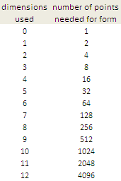
| Dimension | Vertices |
|---|---|
| 0D | 1 |
| 1D | 2 |
| 2D | 4 |
| 3D | 8 |
| 4D | 16 |
| 5D | 32 |
Each step doubles the structural complexity of the coordinate system.
Dimensions and the Definition of Form
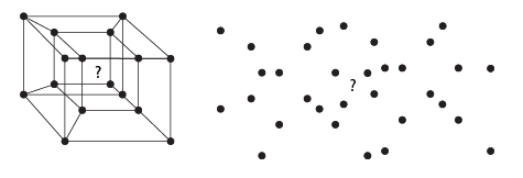
A single point does not allow form to be described. Geometry emerges only when relationships between points exist.
- 0 dimensions → a single point
- 1 dimension → a line defined by two points
- 2 dimensions → a plane defined by four vertices
- 3 dimensions → a cube defined by eight vertices
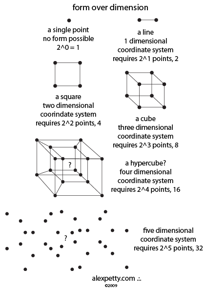
Higher dimensional analogues follow the same pattern. A 4 dimensional hypercube contains 16 vertices and a 5 dimensional one contains 32.
This doubling relationship appears repeatedly in mathematics whenever dimensional structure increases.
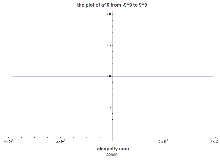
The Zero Dimension Case
A familiar identity in algebra is
$a^0 = 1$
This follows directly from the standard rules of exponents. Although elementary, it highlights an interesting structural feature. Raising a number to the zero power removes the influence of the base and produces the same result regardless of magnitude.
In other words, once the exponent reaches zero, differences in size disappear and the result becomes invariant.
By itself this identity is straightforward. It becomes more interesting when considered alongside dimensional growth. If higher powers correspond to geometric extension such as lines, squares, and cubes, then the zero power case can be thought of as the limiting condition in which no geometric extension occurs at all.
From that perspective the expression $a^0 = 1$ represents a system without dimensional extension. Only a single value remains.
This interpretation is not meant as a physical claim. It simply provides a useful starting point for examining how powers behave when their values are reduced under modulus 9 arithmetic in the tables that follow.
Zero Dimensional Growth
The following diagram illustrates how values behave when numbers raised to the zero power are examined under modulus 9 reduction.
Reducing these values modulo 9 produces the following table.
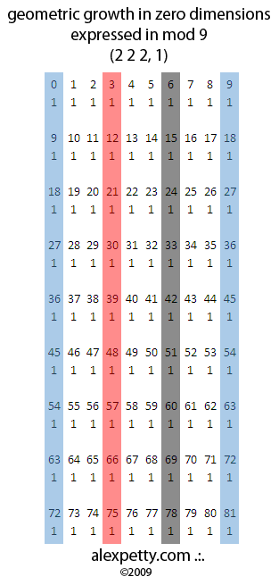
To summarize the structure of the table two simple quantities can be defined.
Growth Signature (GS)
The Growth Signature is derived from the sums of selected column pairs reduced modulo 9.
Increment Line Sum (ILS)
The Increment Line Sum is the digit sum of each row reduced modulo 9.
In this zero dimensional case the values collapse to a uniform structure. All entries reduce to the same value which produces a Growth Signature of 2 2 2 and an Increment Line Sum of 1.
One Dimensional Growth
The familiar visualization of one dimensional growth is shown below.
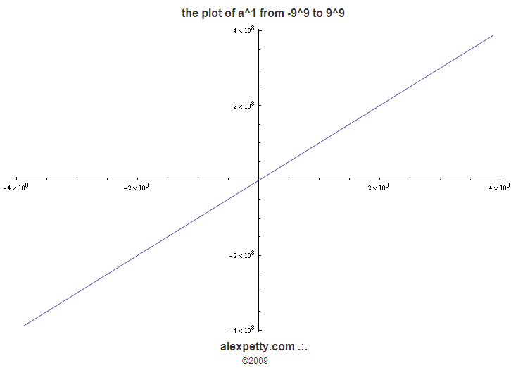
When sequential numbers raised to the power of one are reduced modulo 9 the resulting structure is
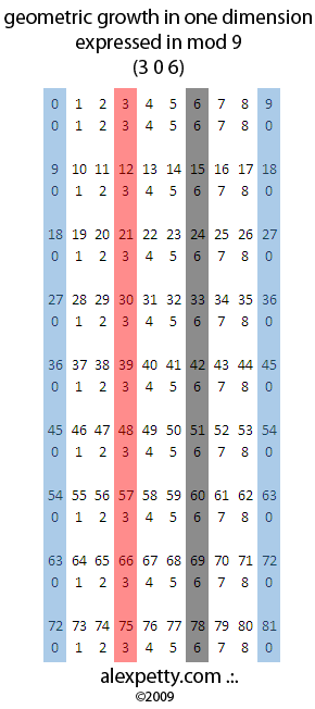
In this case the system behaves linearly. Certain positions remain fixed within the sequence while others cycle through predictable patterns.
For this table the values are
- GS = 3 0 6
- ILS = 0
An interesting property of modulus 9 arithmetic is that the digit sequence used to compute the ILS repeats identically in every increment of nine.
Two Dimensional Growth
The geometric interpretation of second dimension growth corresponds to squares.
When squares are reduced modulo 9 the following table appears.
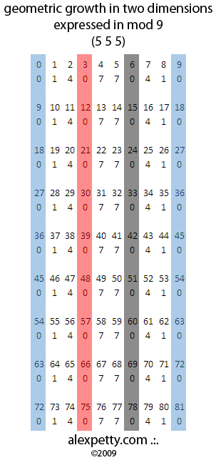
In this case several positions collapse to zero while others produce a palindromic pattern.
One of the sequences produced is
1 4 7 7 4 1
This symmetry appears naturally in square growth under modulus 9 reduction.
The key values for this table are
- ILS = 24 → 6 (mod 9)
- GS = 5 5 5
Three Dimensional Growth
The geometric interpretation of third dimension growth corresponds to cubes.
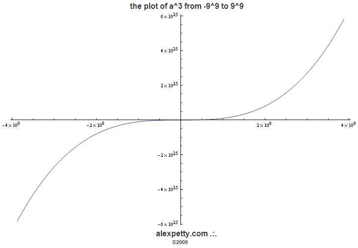
Reducing cubic growth modulo 9 produces the following structure.
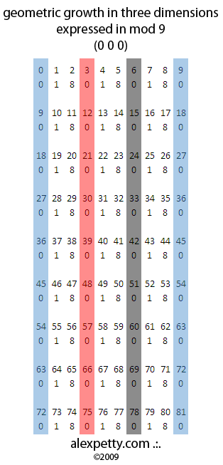
Here the structure simplifies considerably.
- GS = 0 0 0
- ILS = 0
Interpreting the Tables
Before examining these tables it is helpful to recall that reducing numbers by repeated digit sums is equivalent to computing residues modulo 9. The patterns that appear therefore reflect the structure of powers in modular arithmetic.
For example
625 → 6 + 2 + 5 = 13 → 1 + 3 = 4
which corresponds to
625 mod 9 = 4
Because of this relationship the digit sum reduction used throughout these tables is simply another way of expressing arithmetic modulo 9.
Cycles in Powers
When powers of numbers are examined modulo a fixed base repeating cycles appear naturally. This is a standard feature of modular arithmetic. The residues of powers eventually repeat.
For example when squares are reduced modulo 9 we obtain the repeating sequence
1, 4, 7, 7, 4, 1
Cubes produce another repeating pattern. These cycles arise because only a limited number of residues exist modulo 9 so repeated multiplication must eventually revisit earlier values.
Increment Line Sum
To summarize the structure of each table the Increment Line Sum (ILS) can be defined as the sum of all entries in a given row reduced modulo 9.
Mathematically this is simply
ILS = (sum of row values) mod 9
Because each row represents a sequence of numbers raised to a fixed power the ILS highlights how the overall structure evolves as the exponent changes.
Interestingly the ILS values oscillate between 0 and 6 across dimensions.
Growth Signature
A second quantity that summarizes the structure of the table is the Growth Signature (GS). This value is obtained by grouping selected columns and summing their entries modulo 9.
Although the definition is simple the resulting patterns show a repeating sequence across higher powers.
0 0 0 → 8 8 8 → 6 0 3 → 2 2 2 ← 3 0 6 ← 5 5 5 ← 0 0 0
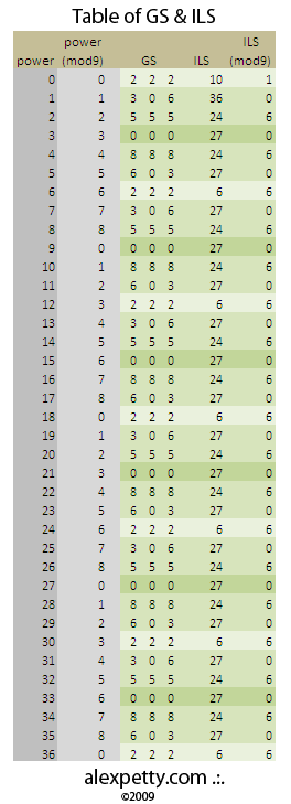
This repeating structure arises from the behavior of power residues modulo 9.
Closing Thoughts
The purpose of these diagrams is not to introduce new arithmetic rules but to visualize familiar operations in a different coordinate framework.
When powers of numbers are examined through modular reduction and arranged across dimensions repeating structures and symmetries appear that are not immediately visible in ordinary numerical tables.
It is also worth noting that there is nothing inherently special about base 10 itself. Any numeral system will produce its own modular cycles when arithmetic is examined in this way. However because our notation and everyday calculations are built around base 10 the patterns produced under modulus 9 reduction are particularly easy to observe.
Whether these structures correspond to deeper geometric or algebraic invariants remains an open question. At the very least they illustrate how even simple arithmetic operations can reveal additional order when viewed through different mathematical lenses.
.:.