Long Division and Euclid’s Lemma
Most of us first encountered long division in grade school. At the time it likely appeared to be nothing more than a mechanical process used to divide one number by another.
But long division is far more than a classroom arithmetic trick.
What we call long division is actually an implementation of the Division Algorithm, a procedure that traces its origins back to ancient Greek mathematics and is closely related to a foundational theorem known as Euclid’s Division Lemma. This lemma guarantees that any integer can be uniquely decomposed into a quotient and a remainder.
In other words, long division is not merely a computational shortcut. It is a window into the internal structure of integers.
One of the most remarkable aspects of long division is that it allows us to examine numbers with arbitrary precision. Unlike floating point calculations, which introduce approximations, the division algorithm lets us analyze number relationships exactly and extend those relationships indefinitely.
This makes long division an extremely powerful conceptual tool. Behind the familiar pencil-and-paper procedure lies one of the key structural properties of the integers: every integer can be expressed uniquely as
$a = bq + r$
where ( q ) is the quotient and ( r ) is the remainder.
This seemingly simple fact has profound consequences. It underlies:
- modular arithmetic
- number theory
- cryptography
- computer arithmetic
- and many modern algorithms
To illustrate the idea concretely, consider a simple example.
Suppose you have 128,654 grains of rice that you want to distribute evenly among 12 people.
The question becomes:
How many times does 12 “go into” 128,654?
In this situation:
- 12 is the divisor
- 128,654 is the dividend
- the number of times 12 can be distributed is the quotient
- anything left over is the remainder
Long division provides a systematic method for determining these values.
The procedure works digit by digit, progressively revealing the structure of the number being divided.
Below is the process step by step.
Division as a Structural Process
It is easy to overlook how remarkable the division algorithm actually is.
When we perform long division we are not merely computing a number. We are progressively revealing the internal structure of the dividend.
The procedure works digit by digit. At each step we determine how many copies of the divisor can fit into the portion of the number currently under consideration. Whatever cannot fit becomes the remainder that is carried forward into the next step.
In this way division recursively decomposes the number, layer by layer.
Each step exposes another digit of the quotient and another piece of the number’s structure.
What makes this especially interesting is that the process can continue indefinitely. If the remainder never becomes zero, we can append additional zeros and continue the procedure forever. The algorithm therefore allows us to examine the ratio between two numbers to any arbitrary level of precision.
In this sense long division acts like a mathematical probe. It lets us explore the relationship between numbers with whatever resolution we choose.
A Quiet but Powerful Property
The division algorithm has another subtle but powerful property.
At every stage of the procedure, the remainder is constrained within a very small range:
$0 \le r < b$
]This means the remainder always lives inside a bounded interval determined by the divisor.
No matter how large the dividend becomes, the remainder can only take on a limited set of values.
This simple restriction is what makes the algorithm so stable and predictable. It guarantees that each step in the process produces exactly one new digit in the quotient.
And because Euclid proved that the quotient and remainder are unique, the structure revealed by long division is not arbitrary. It is intrinsic to the numbers themselves.
Division as a Window into Number Structure
When we begin to look at division this way, it becomes clear that the algorithm is doing something deeper than performing arithmetic.
It is factoring a number into layers of scale.
Each digit in the quotient corresponds to a multiple of the divisor at a particular power of ten. The algorithm is therefore navigating through the place-value hierarchy of the number system.
In effect, division is tracing a path through the number’s positional structure.
Seen from this perspective, long division is not simply a schoolroom technique. It is a method for navigating the architecture of the integers.
A Question Worth Asking
This observation suggests an interesting question.
If the division algorithm exposes structural relationships within numbers, might there be patterns hidden within the combinations of quotients and remainders themselves?
In other words, if we systematically examine the quotient–remainder pairs produced by Euclid’s lemma across many values, do recognizable structures begin to appear?
This question led me to construct the following charts, where the values of Euclid’s division lemma are arranged and examined through the lens of Foundational Mathematics.
Mapping the Quotient–Remainder Structure
To explore this idea further, I constructed a simple experiment.
Instead of examining a single division problem at a time, I generated the full set of quotient–remainder results produced by Euclid’s division lemma for many small integers.
In this case I examined the combinations that arise when:
- the dividend (a) ranges from 1 through 9, and
- the divisor (b) ranges from 0 through 9.
For each pair ((a,b)) the division lemma produces a unique pair ((q,r)) satisfying
$a = bq + r \qquad \text{with} \qquad 0 \le r < b$
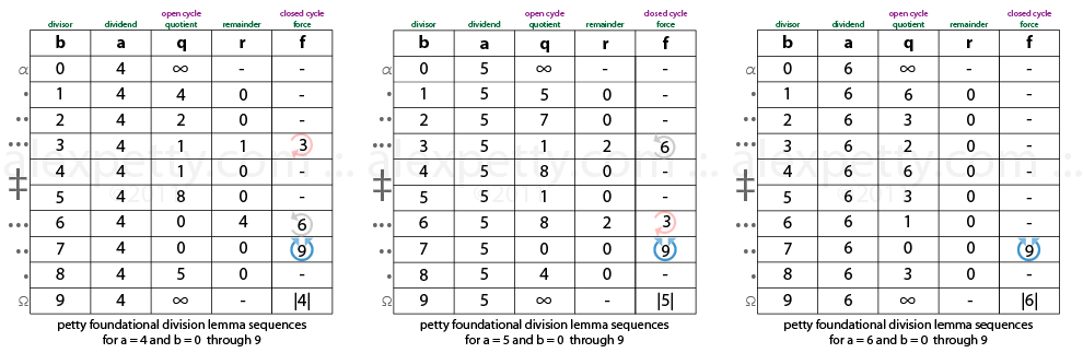
Plotting these results in tabular form produces the matrix shown below.
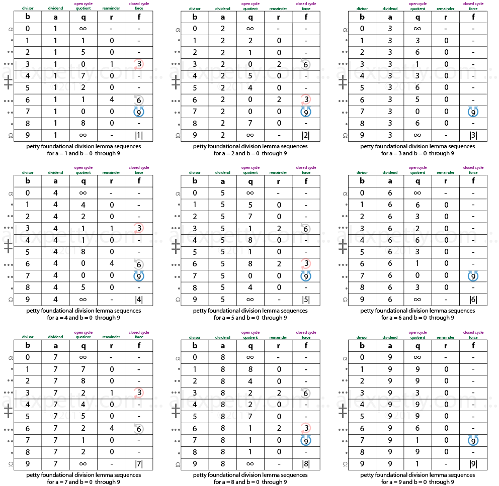
Quotient–remainder structure for small integers
At first glance the chart appears to be nothing more than a simple table of arithmetic results.
However, when the values are examined collectively, a number of regularities begin to appear.
The quotients and remainders do not distribute randomly. Instead they form recognizable patterns that repeat and propagate across the table.
These repeating structures suggest that the division process is revealing deeper organizational properties of the integers.
Compression and Radial Structure
One way to visualize these patterns is through radial compression.
If we repeatedly compress numbers by summing their digits until only a single digit remains, many of the values in the matrix fall onto repeating radial lines.
For example:
$546 \rightarrow 5+4+6 = 15 \rightarrow 1+5 = 6$
Thus the number 546 lies on the 6 radial.
This form of compression causes numbers that appear very different at first glance to collapse back onto a small set of underlying generators.
When the results of the division lemma are examined under this compression, the patterns in the chart become easier to see.
The Role of Zero and Nine
Another interesting observation emerges from this compression process.
Within the decimal system the numbers 0 and 9 behave like boundary values.
They mark the beginning and end of the cycle.
This is illustrated in the diagram below.
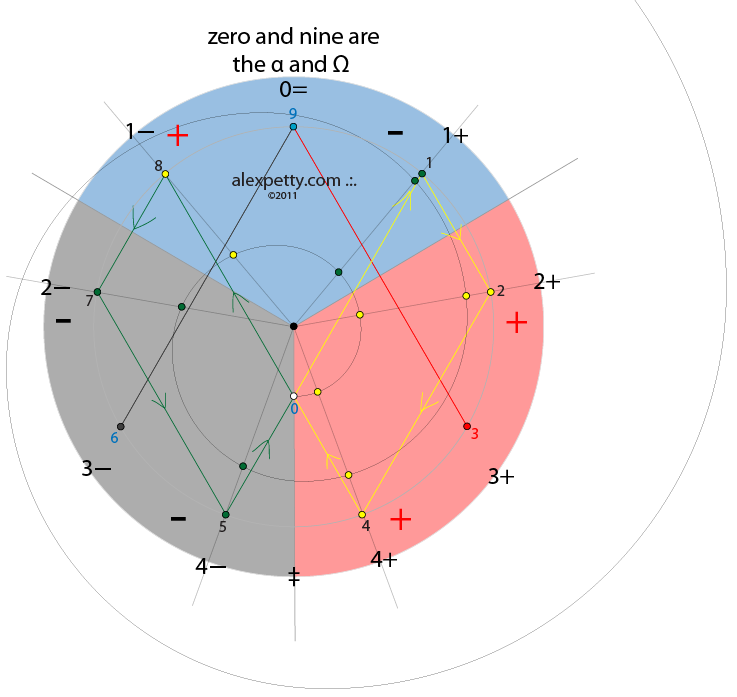
In this representation, zero and nine serve as the endpoints of a repeating numerical cycle.
Each time the sequence expands outward it eventually compresses back toward its radial origin.
A Speculative Question
These observations naturally lead to a broader question.
If Euclid’s division lemma provides the structural rule governing how integers decompose into quotient–remainder pairs, could a compressed radial representation provide a complementary way of visualizing those relationships?
In other words, might there exist a systematic way to navigate the structure of numbers using these compression patterns?
A Structural Reflection
When numbers are examined through repeated compression, a small set of values begins to dominate the structure.
In the decimal system the values 0 through 9 define the entire numerical landscape. Every larger number can be understood as a recombination of these fundamental digits.
When compression is applied repeatedly, the sequence collapses back toward this basic set again and again.
In this sense, the digits behave like generators from which larger numerical structures emerge.
Cycles Within the Decimal System
Within this framework, certain digits appear to play particularly distinctive roles.
The numbers 3, 6, and 9 often appear as pivot points in cyclic numerical behavior. Meanwhile the sequence
$1,2,4,8,7,5$
tends to form repeating cycles under various multiplicative processes.
These observations have been noted by many investigators of numerical patterns. They do not change the underlying mathematics, but they can provide a helpful way to visualize how number sequences evolve.
Alpha and Omega
In the compressed representation shown earlier, the values 0 and 9 appear as boundary markers.
Zero represents the neutral origin of the number system, while nine represents the completion of a cycle before the sequence rolls over into the next order of magnitude.
In that sense, the pair can be viewed symbolically as the beginning and end of a numerical cycle.
Every new order of magnitude simply restarts the same structural process at a higher scale.
A Broader Perspective
The deeper lesson here is not that numbers possess mystical properties, but that simple mathematical rules often generate surprisingly rich patterns.
The division algorithm reveals one aspect of this structure by decomposing numbers into quotient–remainder pairs.
Radial compression reveals another by showing how seemingly complex numbers collapse back onto a small set of repeating generators.
Taken together, these views remind us that the familiar arithmetic we learn in childhood contains far more structure than it first appears.
Even something as ordinary as long division can open a window into the deeper architecture of the integers.
.:.