The Golden Ratio

An origin essay from January 2010, revisited in September 2026.

Divide one into three equal parts. There are more pieces to count, but the amount is still one. This reciprocal view of number interested me from the start. Three gave me thirds, five gave me fifths, and the whole stayed in the account.

The golden ratio gave that interest a particular focus. A whole can divide into two unequal shares so that the proportion between the shares repeats the proportion between the whole and its larger share. We can make the same division again inside a smaller piece. The relationships continue while the pieces still account for the original one.

That was the question behind these drawings. I wanted to understand how a number could describe a division, how a proportion could survive a change of scale, and how to keep the whole visible through both.

Number through its reciprocal

The little drawing below puts the change of viewpoint plainly. Across the top are three separate units. Below is one unit divided into thirds.

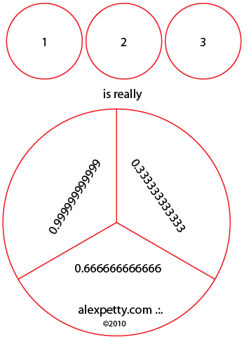
The lower picture asks us to count parts of a fixed whole. Each part has size one third. Add the three shares and we are back at one.

For any positive integer $n$, the same accounting gives $n$ shares of size $1/n$.

$$n\cdot\frac1n=1.$$

Increasing the number of parts makes each part smaller. The reciprocal tells us how much smaller. This became a useful way for me to look at an integer, through the divisions it makes within unity.

One whole, two unequal shares

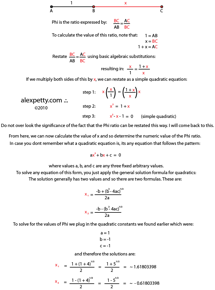
Now divide a line into a longer part and a shorter part. Require the whole divided by the longer part to equal the longer part divided by the shorter part.

In my original pentagon drawing, B makes that division on the diagonal AC. The longer segment is BC, and the shorter is AB. Their ratio is the golden ratio, written $\varphi$.

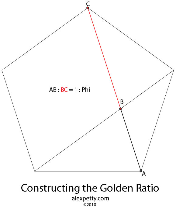
Let the shorter piece have length one. The longer then has length $\varphi$, and the whole has length $1+\varphi$. The repeated proportion gives

$$\varphi^2=\varphi+1,\qquad \varphi=\frac{1+\sqrt5}{2}\approx1.618034.$$

Normalize the whole to one instead. The longer piece now occupies $1/\varphi$ of it, and the shorter occupies $1/\varphi^2$.

$$\frac1\varphi+\frac1{\varphi^2}=1.$$

About 0.618 of the whole lies on one side of the cut and 0.382 on the other. This is the form that matters most to me here. The golden proportion has become a division of unity.

Division without loss

Take the shorter piece and divide it in the same proportion. Keep the larger piece from that division, then divide the new remainder again.

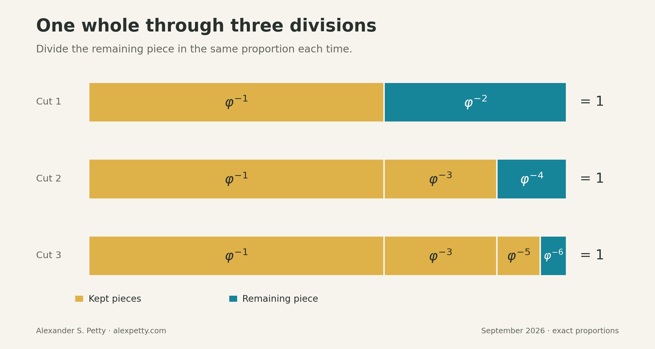
After the second cut, the three lengths are $\varphi^{-1}$, $\varphi^{-3}$, and $\varphi^{-4}$. After the third, they are $\varphi^{-1}$, $\varphi^{-3}$, $\varphi^{-5}$, and $\varphi^{-6}$. Each row still sums to one.

The remainder is part of the account at every finite step. As we continue, it shrinks toward zero. The pieces set aside then fill the unit in the limit.

$$\varphi^{-1}+\varphi^{-3}+\varphi^{-5}+\cdots=1.$$

This gives the conservation I had in mind a simple arithmetic form. We can refine the division without losing any of the whole. The golden ratio supplies one particularly economical rule for doing it.

The same split is present in the original golden triangle. In the drawing below, D lies on AC. Drawing BD divides triangle ABC into two smaller regions.

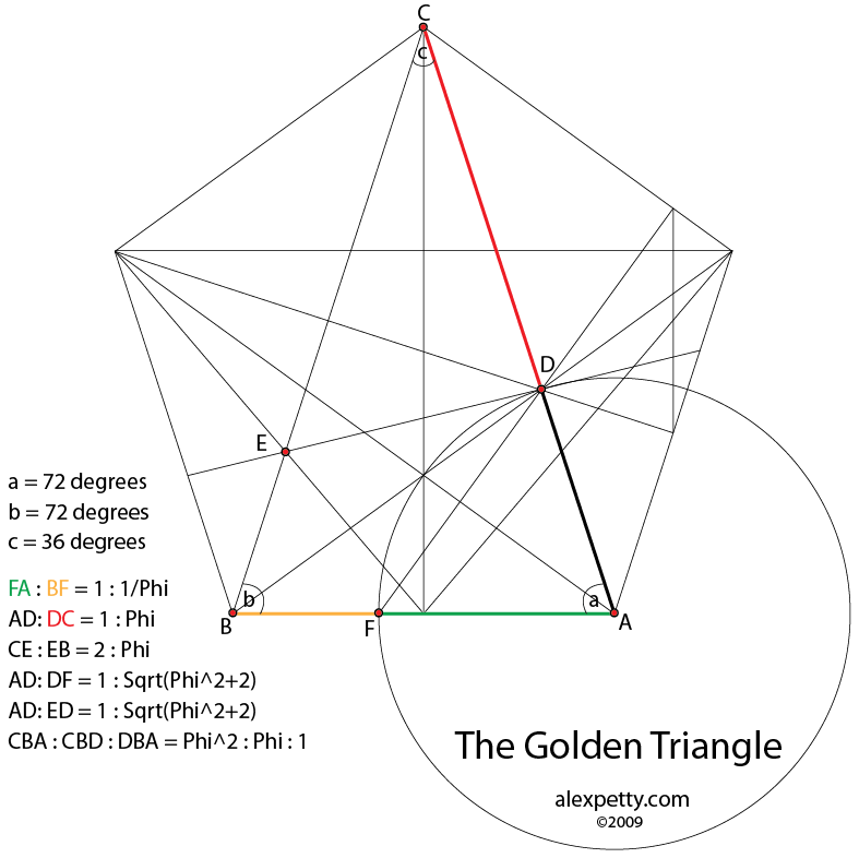
The two regions share the same altitude from B to the line AC, so their areas divide in the same proportion as CD and DA. Give the whole triangle area one and the parts again have areas $1/\varphi$ and $1/\varphi^2$. The line-segment identity is doing work inside the more elaborate drawing.

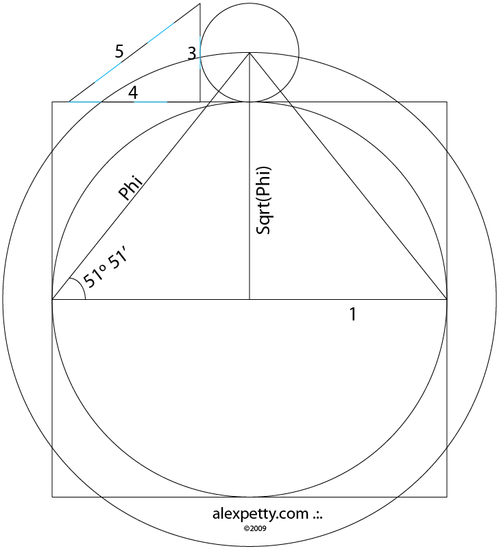
Read the original algebra and right-triangle constructions

Fibonacci proportions

The Fibonacci sequence provides a way to approach the same division using integers. Start with one and one, then keep adding the previous two numbers.

1, 1, 2, 3, 5, 8, 13, 21, 34, 55, 89, 144, …

Take five and eight. Together they make thirteen, so within a unit their shares are $5/13$ and $8/13$. Take eight and thirteen next. Their shares are $8/21$ and $13/21$. At every stage the two fractions sum to exactly one.

The larger share approaches $1/\varphi$, and the smaller approaches $1/\varphi^2$. The partition is exact at each step even while its proportions are still changing.

The ratios of successive Fibonacci numbers explain the convergence. If a ratio is $R$, the next one is $1+1/R$. A limiting ratio must therefore satisfy $R=1+1/R$, which gives the same quadratic as the line segment.

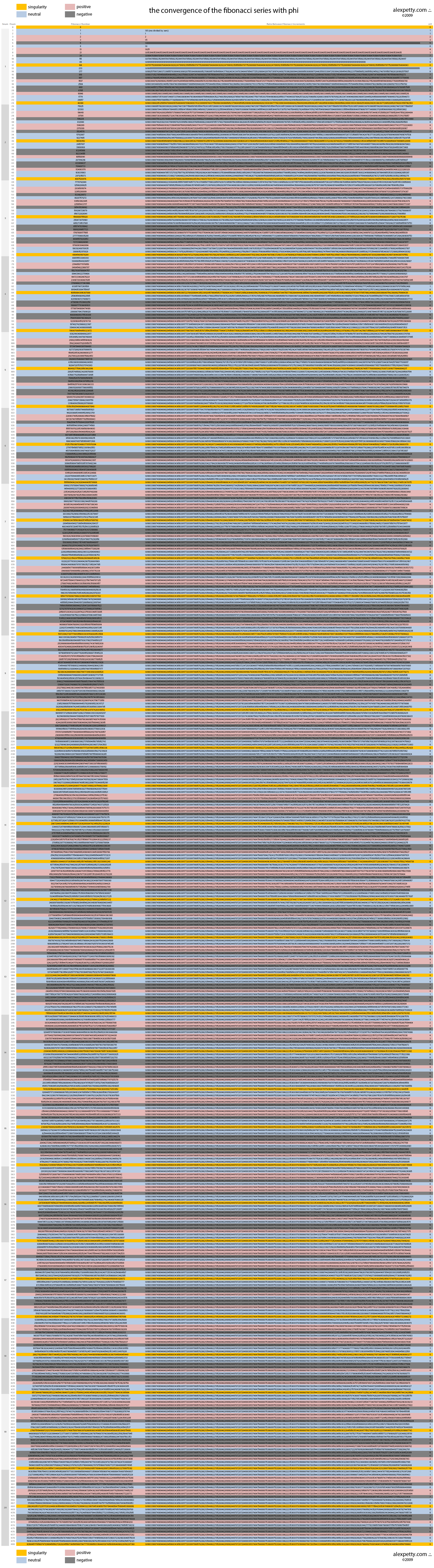
The original tables follow the calculation much farther than a few rounded decimals. The second sheet is especially revealing. Although I called it an error table, it records phi divided by the current Fibonacci ratio. Its reference value is one.

Fibonacci ratio	Decimal value	Phi divided by that ratio
2/1	2.000000	0.809017
3/2	1.500000	1.078689
5/3	1.666667	0.970820
8/5	1.600000	1.011271
13/8	1.625000	0.995713
21/13	1.615385	1.001640

The last column alternates around one. Subtract one from it to get a signed discrepancy that approaches zero. The old sheet keeps the multiplicative comparison intact, making the return toward unity visible in the digits.

Inspect both original Fibonacci tables at full resolution

The alternation has an exact algebraic source. The quadratic has two roots, $\varphi$ and $-1/\varphi$. With $F_0=0$ and $F_1=1$, the discrepancy between the next Fibonacci number and phi times the current one is

$$F_{n+1}-\varphi F_n=\left(-\frac1\varphi\right)^n.$$

The negative reciprocal changes the sign at every step and reduces the magnitude. It belongs to the same equation as the growing ratio. The drawings gave me a reason to inspect that smaller contribution instead of rounding it away.

A cycle needs its whole state

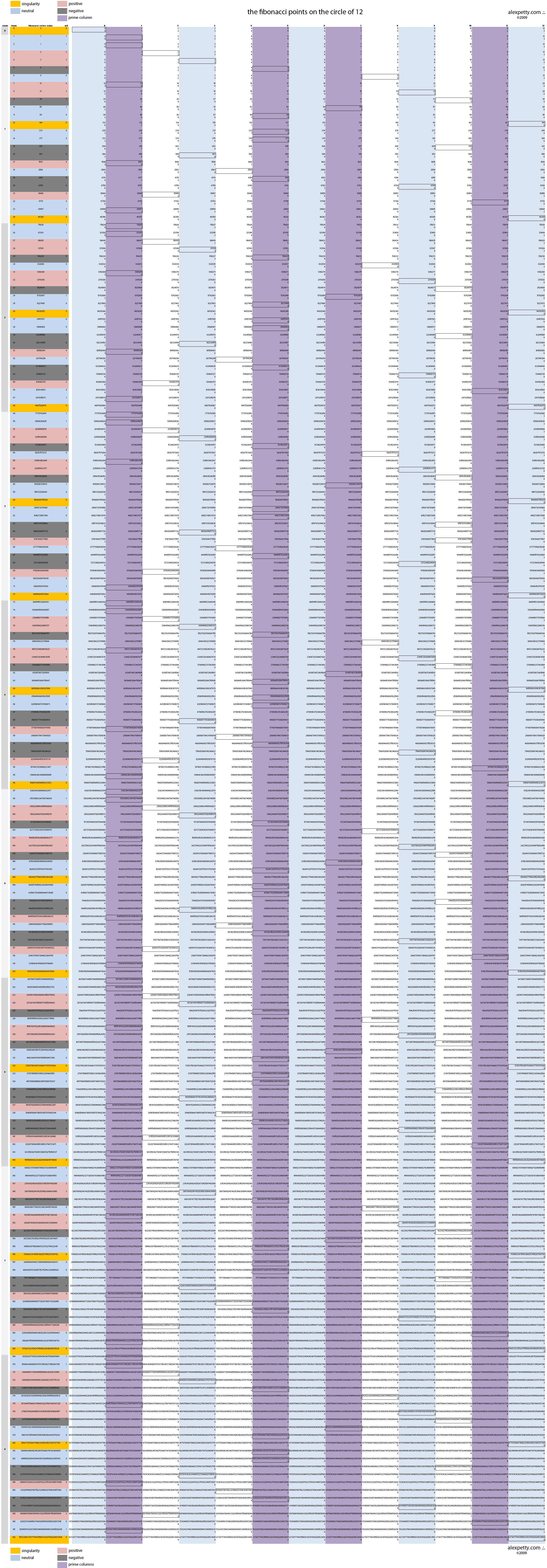
The circle-of-twelve sheets make another comparison. They place each Fibonacci number in its column modulo twelve, while retaining its modulo-nine classification at the left. The integers grow, but these remainder coordinates can return to an earlier state.

Zero returns after twelve Fibonacci steps. That alone does not restart the sequence. The recurrence needs two consecutive values.

Step	Fibonacci value modulo 12	Next value modulo 12
0	0	1
12	0	5
24	0	1

At step twelve, zero is followed by five. At step twenty-four, the original pair zero and one returns. The entire pattern then repeats. The Fibonacci sequence modulo nine also has period twenty-four, so both readings fit into the same repeating arrangement.

Explore the two original circle-of-twelve sheets

The return is guaranteed for the pair of Fibonacci residues under any fixed modulus. There are only finitely many pairs, and subtraction recovers the previous pair from the next one. The process is reversible, so the starting pair lies on a cycle.

That distinction between a repeated value and a complete returning state became useful well beyond these particular drawings.

Fractions as a portrait of an integer

The reciprocal view also suggested a way to examine a denominator in full. Put every fraction from $1/n$ through $(n-1)/n$ inside the unit interval and read their expansions together.

For seven, the six interior fractions in decimal give

1/7 = 0.142857…
2/7 = 0.285714…
3/7 = 0.428571…
4/7 = 0.571428…
5/7 = 0.714285…
6/7 = 0.857142…

Each line repeats its displayed six-digit block. All six blocks are rotations of one another. Long division carries a remainder from one place to the next, and these six starting fractions enter the same cycle at different points.

The fractions pair across the middle of the unit. One seventh and six sevenths add to one, as do two sevenths and five sevenths, and three sevenths and four sevenths. Their repeating digits pair to nines. The cyclic motion and the complementary pairing are two structures in the same small table.

Changing the denominator or the base can split the fractions into several cycles or make some terminate. That gave me a practical investigation. Keep the whole family in view and compare its internal arrangements. In the later alignment work I began measuring agreement within these fractional fields.

The conserved whole in the later work

The golden algebra returned in Three and the Golden Ratio. There, a specified score counts matching and terminating rows in a fractional field. Its curve meets $1/\varphi$ at the real scale $\varphi^2$. Requiring the crossing scale to be the reciprocal square of the threshold gives a precise condition to study. The golden identity enters that calculation through the stated condition.

The Fibonacci connection also became a tool. Every power of phi reduces to

$$\varphi^n=F_n\varphi+F_{n-1}\qquad(n\ge1).$$

Repetend Rigidity at the Golden Scale uses those coefficients to test possible repeating periods. An algebraic candidate still has to be the length of a cycle that long division can actually produce.

The thread of conservation continues in the cubic-law calculation, where positive reciprocal weights attached to coprime pairs sum to exactly one. The Clocks Beneath Collision Energy groups that mass by period. The remainder clocks move and reset while their shares stay fixed. Period two carries a quarter of the mass; period three carries a sixth.

Those weights are determined by the collision calculation. They are different from the golden shares in the early drawings. The continuing idea is to keep an exact account of the whole while its internal arrangement changes.

That interest was already here. A line, a triangle, a table of fractions, and a long column of decimals gave me different ways to examine it. I still begin by asking how the parts account for one.