The Orbit's Edge

Long division in base two turns $1/243$ into a repeating block $162$ digits long. The remainders behind it wander through $162$ of the numbers below $243$ before they come back to one. A cycle that long looks as if its arithmetic ought to be complicated. Its edge, though, is plain. Line the $162$ remainders up in ordinary order and the set switches off at every multiple of three and back on one step later, the same three-place pattern the whole way around. Every character that responds to that edge needs nothing finer than modulus three. A two-digit rule in base fifteen, with far fewer pieces, spreads its edge over five different moduli. A cycle’s length and the depth of its edge are separate things, and the characters measure the edge.

Carry Boundaries and Bernoulli Spectra in Long Division reduced any finite digit rule to the signed edges of the cells it selects. A repeating tail isn’t a finite digit rule. Its remainders still form a set, though, the orbit that multiplication by the base carves out of the units, and that set has edges in the same sense. The tools are classical, characters, Gauss sums and Jacobi sums. The new part is an exact accounting of the edge’s squared response by conductor, with every level counted as a nonnegative amount, so that nothing at a lower resolution can hide behind a cancellation.

Three steps, four crossings

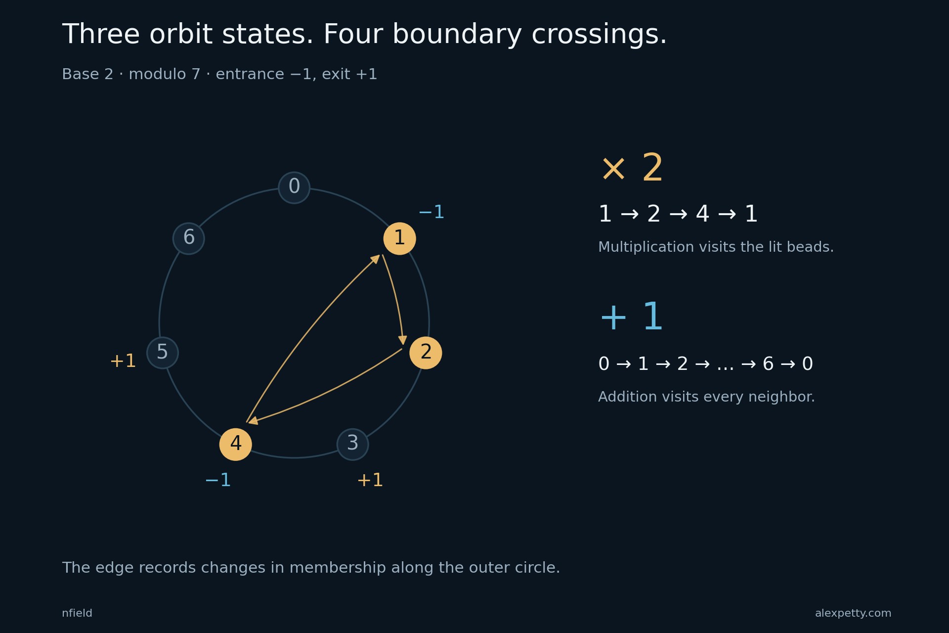
The smallest example is one seventh in base two. Its digits are $0$, $0$, $1$ and then repeat, because the remainders go $1\to2\to4\to1$, doubling each time and subtracting seven whenever they pass it.

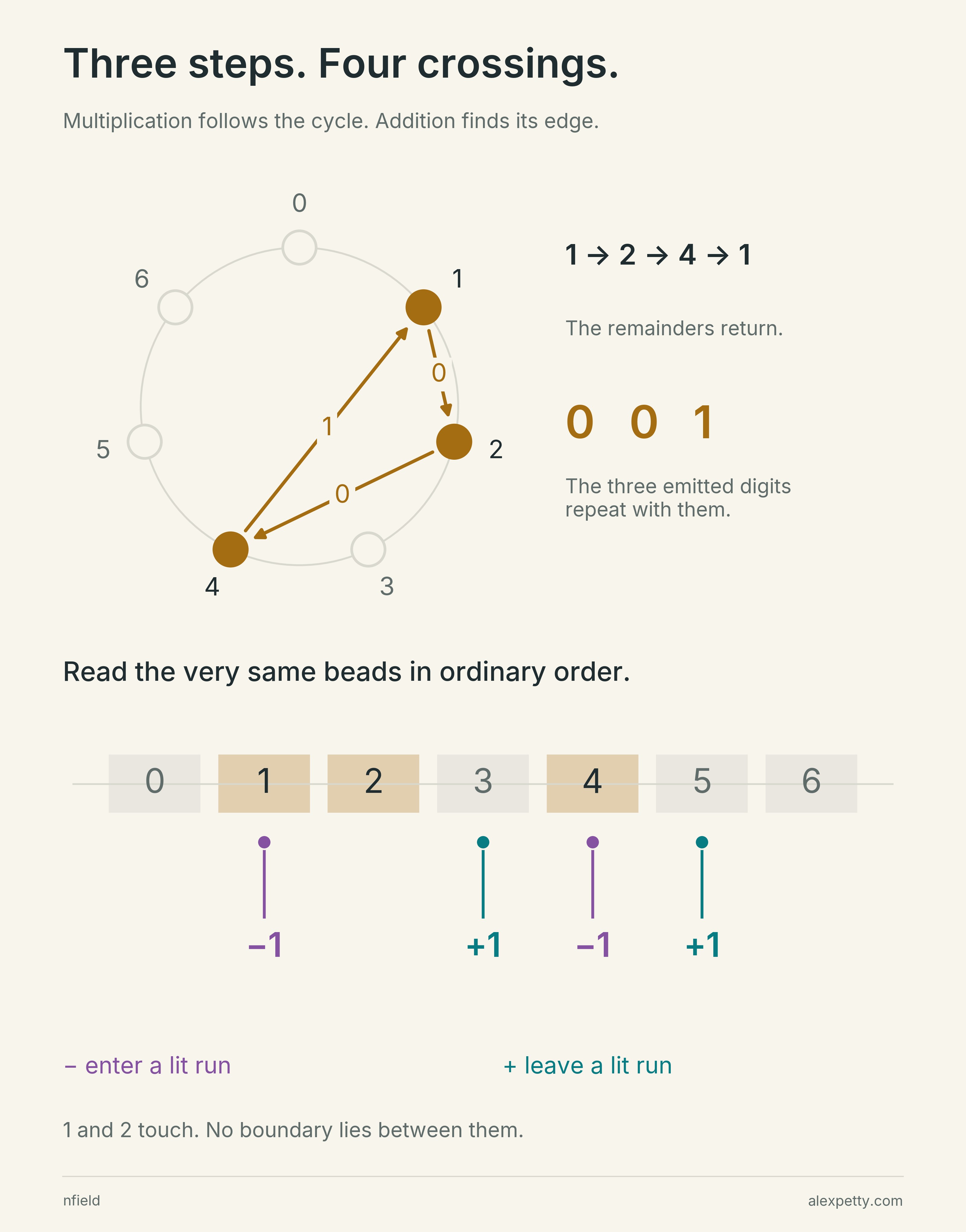
On the circle, the three gold beads are the remainders the cycle visits, joined by the doubling steps and labeled with the digits they write. Below, the same seven beads are laid out in ordinary order as a row of lit and dark cells. The row is dark at $0$, lit at $1$ and $2$, dark at $3$, lit at $4$ and dark at $5$ and $6$. Reading left to right there are four crossings, into the lit cells at $1$ and $4$ and out of them at $3$ and $5$. Multiplication decided which beads are lit. Addition, stepping from each number to the next, finds where the lit set starts and stops, and $1$ and $2$ touch with no crossing between them even though multiplication treats them as separate stops. Give an entrance a minus sign and an exit a plus sign, and the signed edge at seven is minus at $1$, plus at $3$, minus at $4$ and plus at $5$.

The signed boundary and the character measurement

For a base $b$ coprime to $q$, start at remainder one and let $H=\langle b\rangle$ be its multiplicative orbit modulo $q$. Write $\mathbf1_H$ for its membership function. The additive boundary is

$$\mu_H(x)=\mathbf1_H(x-1)-\mathbf1_H(x).$$

For a Dirichlet character $\chi$, its boundary flux is

$$\begin{aligned} S_H(\chi)&=\sum_{x\bmod q}\mu_H(x)\chi(x)\\ &=\sum_{r\in H}\bigl(\chi(r+1)-\chi(r)\bigr). \end{aligned}$$

The second line follows by shifting the first sum by one. Each orbit point contributes the character’s change from that point to its neighbor.

A character is zero on residues that are not invertible modulo $q$. These measurements therefore recover only the boundary restricted to the units. They do not recover the boundary at nonunits. An odd character satisfies $\chi(-x)=-\chi(x)$. Throughout this article, energy means a sum of squared magnitudes $|S_H(\chi)|^2$, without averaging and before applying a Bernoulli factor.

A different invertible starting remainder visits a coset of $H$. The examples and orbit formulas here use the orbit starting at one.

Six remainders, three arrows

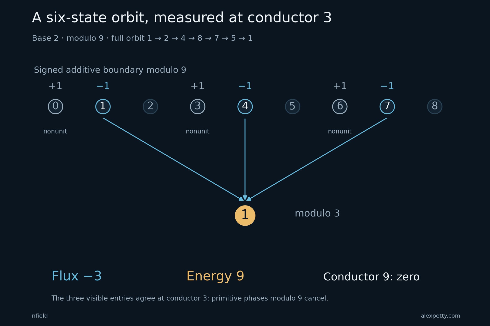
At nine, doubling visits all six remainders that three doesn’t divide before returning,

$$1\to2\to4\to8\to7\to5\to1.$$

In numerical order they form three lit runs, entered at $1$, $4$ and $7$ and left at $3$, $6$ and, wrapping around, $0$.

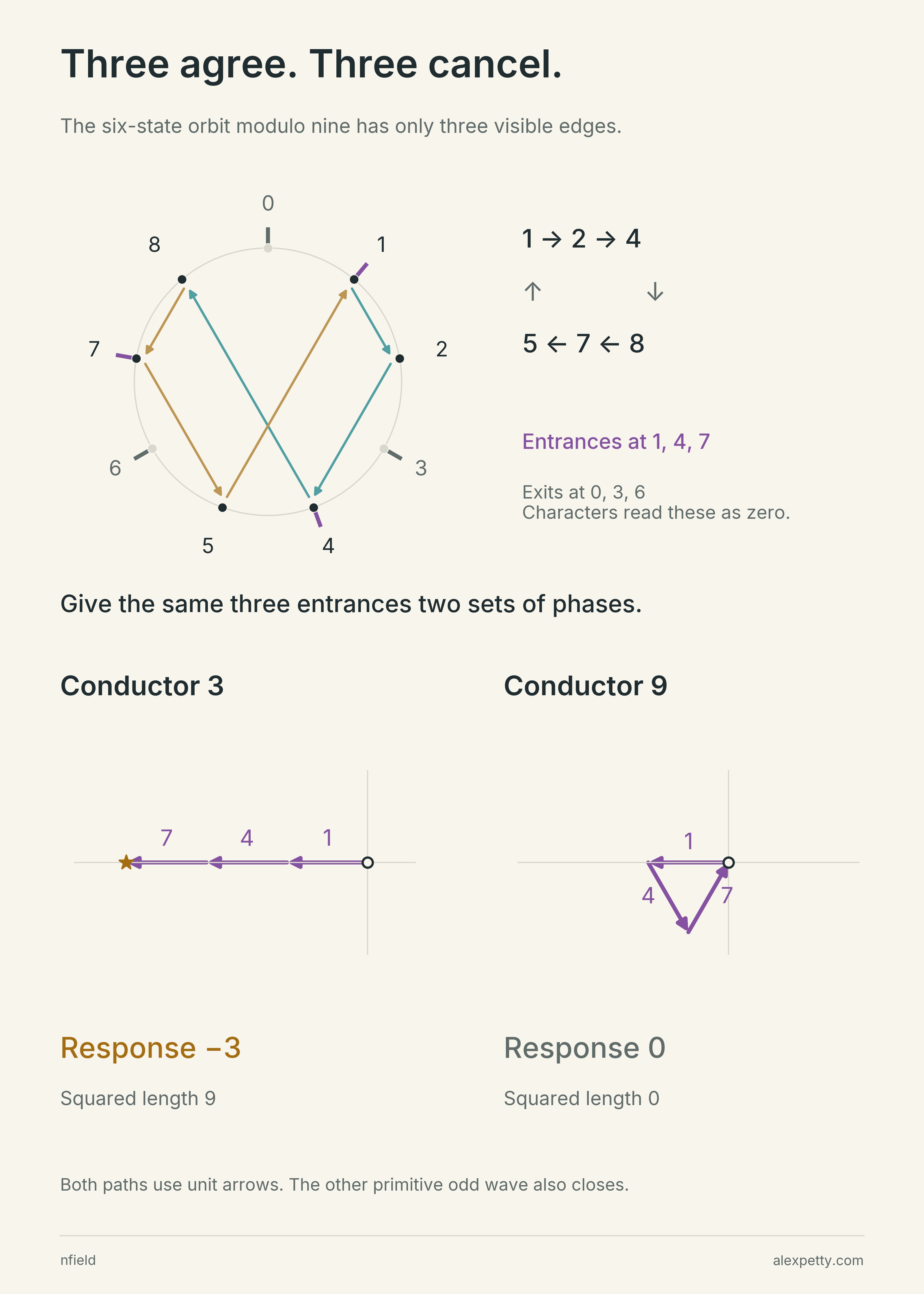
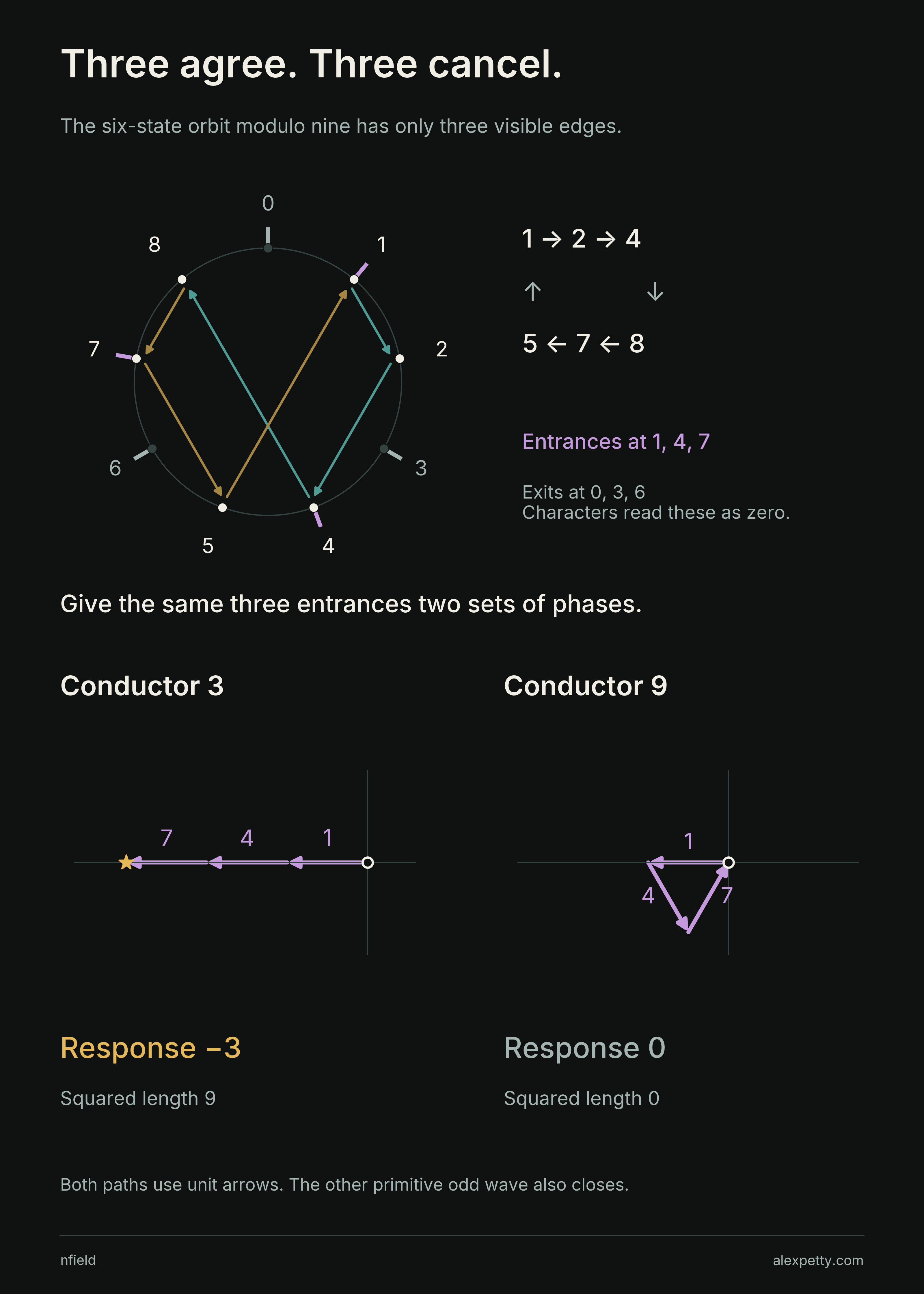
In the figure the violet ticks at $1$, $4$ and $7$ are the entrances and the gray ticks at $0$, $3$ and $6$ are the exits. The exits sit on multiples of three, where every Dirichlet character is zero, so only the three entrances count. Below, two odd characters read them. The character that only sees a remainder modulo three gives $1$, $4$ and $7$ the same arrow, and the three minus signs line up into a response of $-3$, with squared length $9$. A character that needs the full modulus nine turns the three arrows a third of a circle apart, and they close into a triangle with response zero. The other character of that kind closes its triangle the other way. The conductor of a character is the least modulus it needs, and every bit of response in this six-step cycle sits at conductor three.

Both triangles, with the phases written out

The units modulo nine are successive powers of two. Specify a character by

$$\chi_j(2)=e^{2\pi i j/6}.$$

The odd characters have $j=1,3,5$. On the visible boundary $\mu_H=-\delta_1-\delta_4-\delta_7$, their responses are

$$\begin{aligned} S_H(\chi_3)&=-(1+1+1)=-3,\\ S_H(\chi_1)&=-(1+\omega+\omega^2)=0,\\ S_H(\chi_5)&=-(1+\omega^2+\omega)=0, \end{aligned}$$

where $\omega=e^{2\pi i/3}$. The first character factors through modulus three. The other two have conductor nine. Their triangles run in opposite directions and close at the same point.

More stops on the same circuit

Try twenty-seven, then eighty-one, then $243$. Doubling visits $18$, $54$ and $162$ remainders before coming home, and the circles fill with chords as the cycle lengthens.

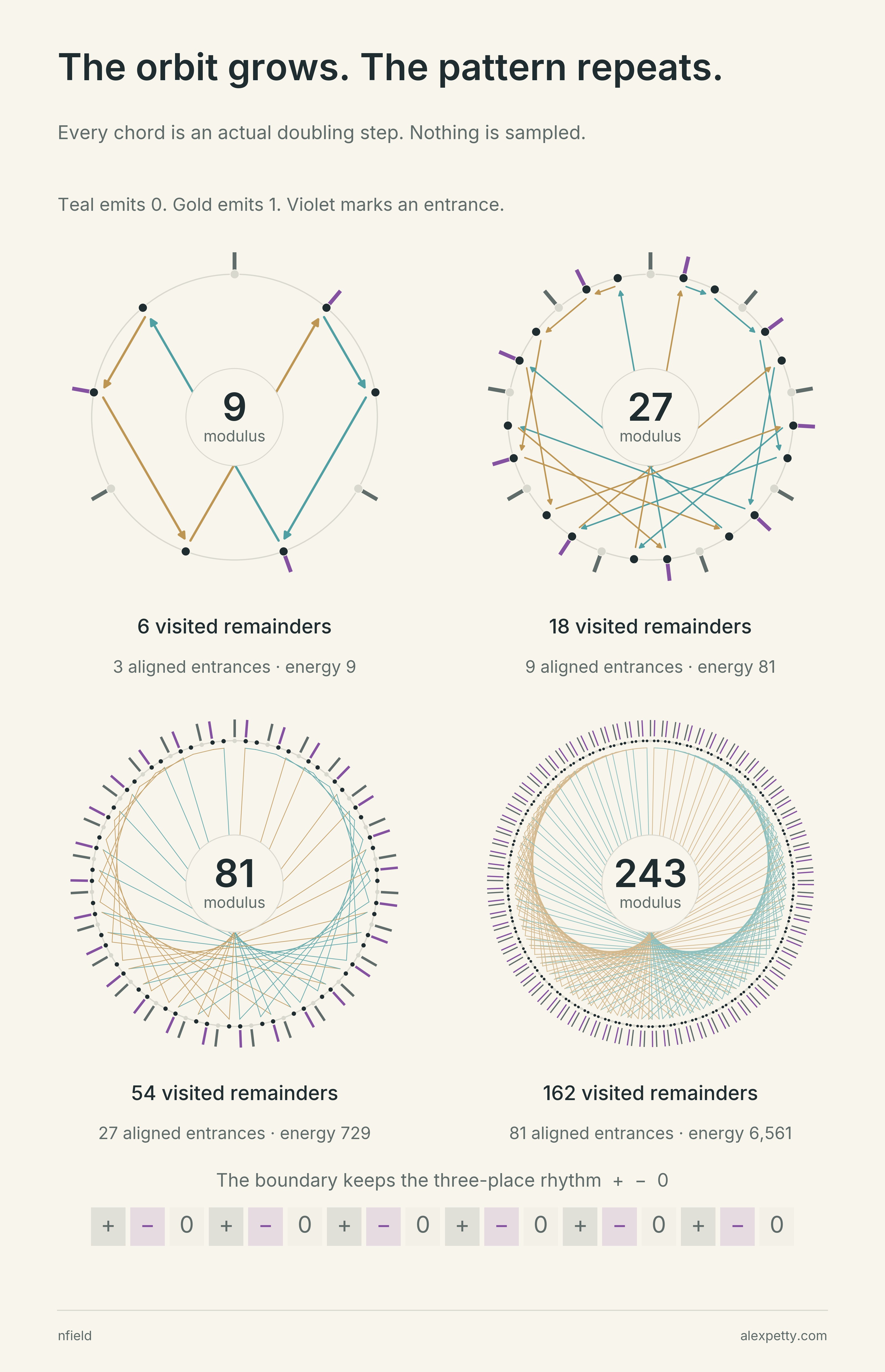
Every chord in the figure is an actual doubling step, all $162$ of them at $243$, and the drawings get busier and busier. The edge doesn’t. Around every circle the entrances and exits keep the three-place rhythm shown along the bottom, an exit at each multiple of three and an entrance one step after it. The energies are $9$, $81$, $729$ and $6{,}561$, which are $3^2$, $9^2$, $27^2$ and $81^2$, the squared number of aligned entrances each time. All of it stays at conductor three. The finer characters keep closing their arrows into polygons. The law is exact for any base whose powers visit every unit modulo an odd prime power, and a base that visits only some of the units can leave a different edge.

The prime-power law, conductor by conductor

Suppose $H=U_{p^e}$ for an odd prime $p$. Membership fails exactly at multiples of $p$, so

$$\mu_H(x)=\mathbf1_{p\mid x}-\mathbf1_{x\equiv1\pmod p}.$$

Characters ignore the first term. At conductor $p$, every one of the $p^{e-1}$ remaining entries has phase one and boundary sign minus one. Each odd character there has flux $-p^{e-1}$.

At a higher conductor $p^f$, the visible residues project onto the subgroup of units congruent to one modulo $p$, with equal multiplicity. A primitive character of conductor $p^f$ is nontrivial on that subgroup, so its sum over the subgroup is zero. This is the same cancellation as the triangle at nine, with more arrows.

There are $(p-1)/2$ odd characters at conductor $p$. Consequently

$$\begin{aligned} P_p&=\frac{p-1}{2}\,p^{2e-2},\\ P_{p^f}&=0\qquad(2\leq f\leq e). \end{aligned}$$

The increasing energy is unnormalized. Both the size of the orbit and the magnitude of its flux grow. The conductor supporting that energy does not.

The energy below 225

Other edges spread out. In base fifteen, the rule asking for a repeated digit in a two-digit word picks the cells $0,16,32,\ldots,224$ out of $225$. A character written modulo $225$ may already be determined modulo $9$ or $25$, so count each odd character at the least modulus it needs and add up the squared responses level by level.

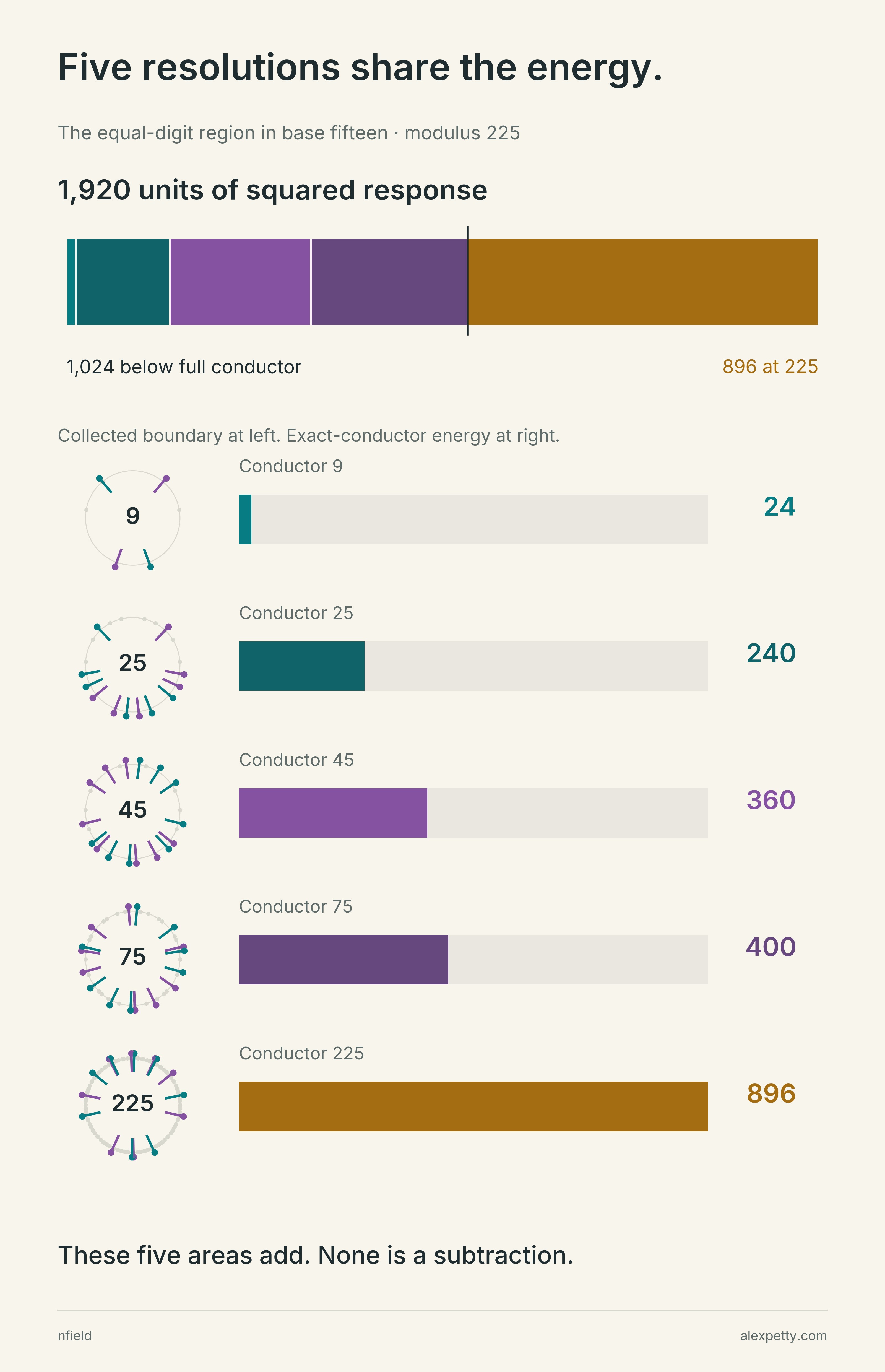
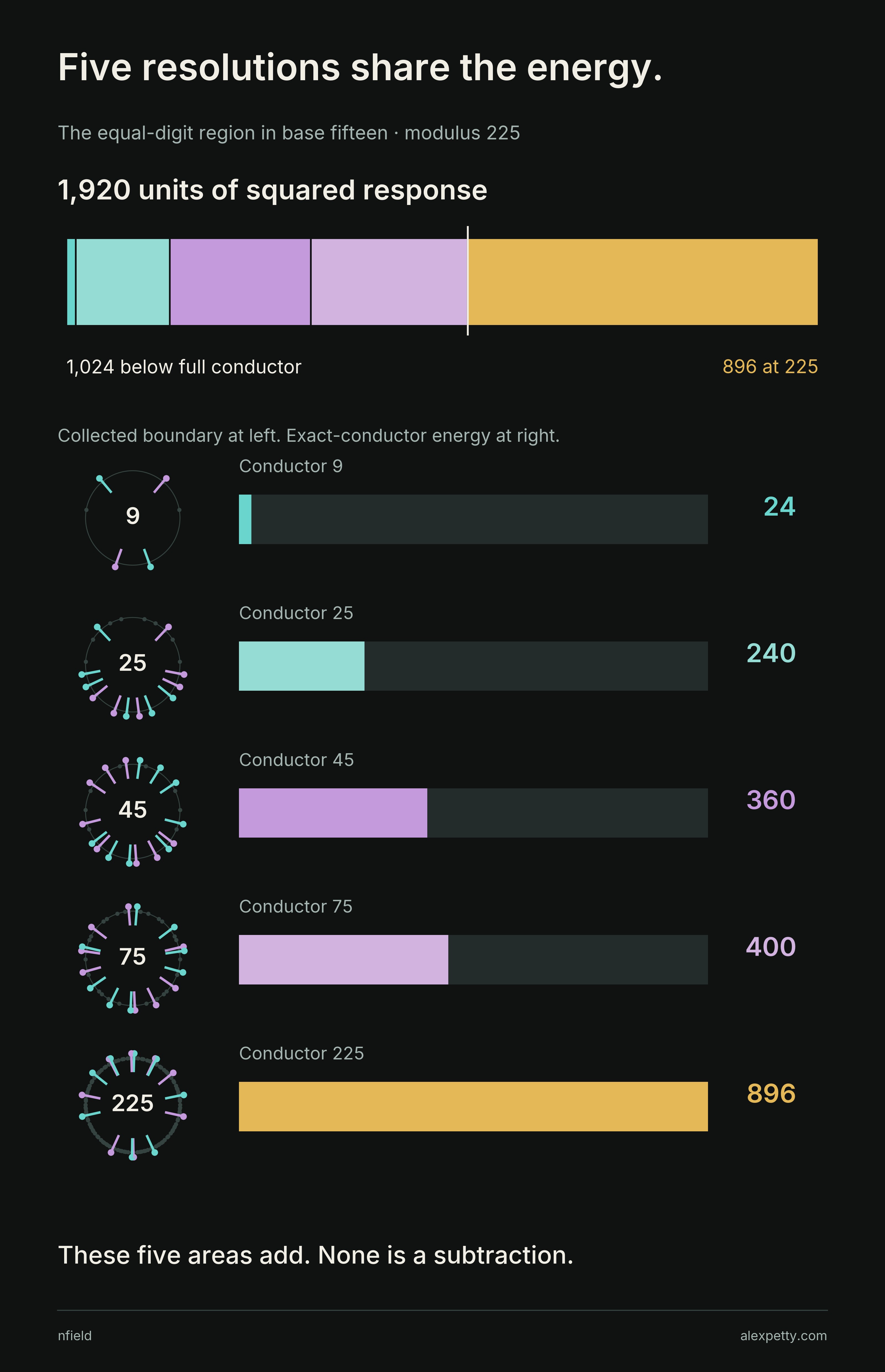
The long bar at the top divides $1{,}920$ units of squared response by area, $896$ at the full conductor $225$ and $1{,}024$ below it. The rows underneath give the five occupied levels, each beside a small ring showing the boundary collected at that modulus. They hold $24$ at conductor nine, $240$ at twenty-five, $360$ at forty-five, $400$ at seventy-five and $896$ at $225$. Every row is a sum of squares, so nothing elsewhere can cancel it. Keeping only the characters that need all of $225$ would miss more than half the energy.

The exact ledger and a boundary that cancels without vanishing

Conductor	Boundary energy
9	24
25	240
45	360
75	400
225	896
Total	1920

To look at a smaller modulus $d$, first restrict the boundary to the units of the original modulus $m$. Then add the weights whose residues agree modulo $d$. Call that collected boundary $M_d$.

$$M_d(r)=\sum_{\substack{x\in U_m\\x\equiv r\pmod d}}\mu(x).$$

Collecting the weights is only the first step. Their arrangement determines which characters can see them. A nonzero collected boundary can still be invisible to every odd character.

In base five, select the two-digit cells whose first digit is smaller than the second. The unit-visible boundary modulo twenty-five consists of four entrances,

$$\mu=-\delta_1-\delta_7-\delta_{13}-\delta_{19}.$$

Modulo five, each of the four nonzero residues receives weight minus one. Opposite residues therefore have equal weights. An odd character gives those residues opposite phases, so their contributions cancel in pairs.

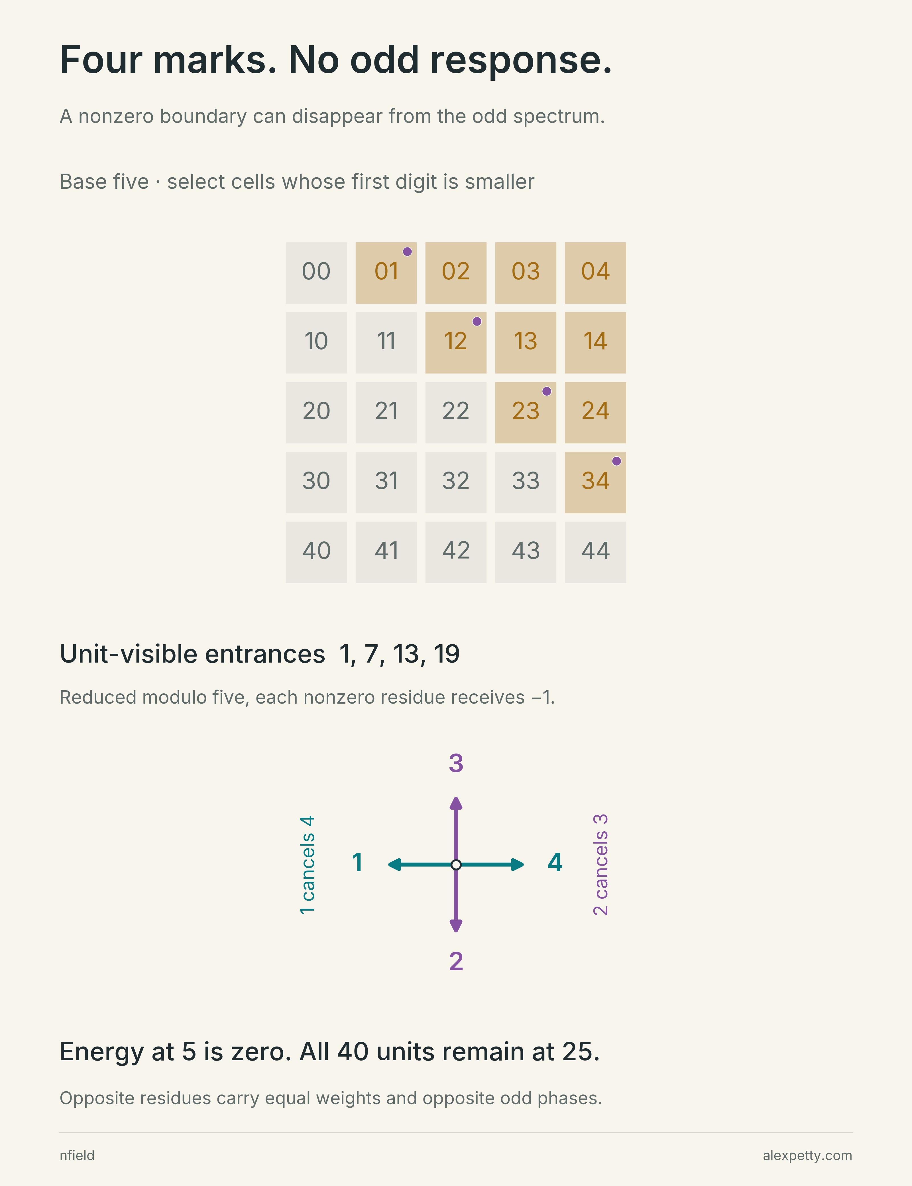
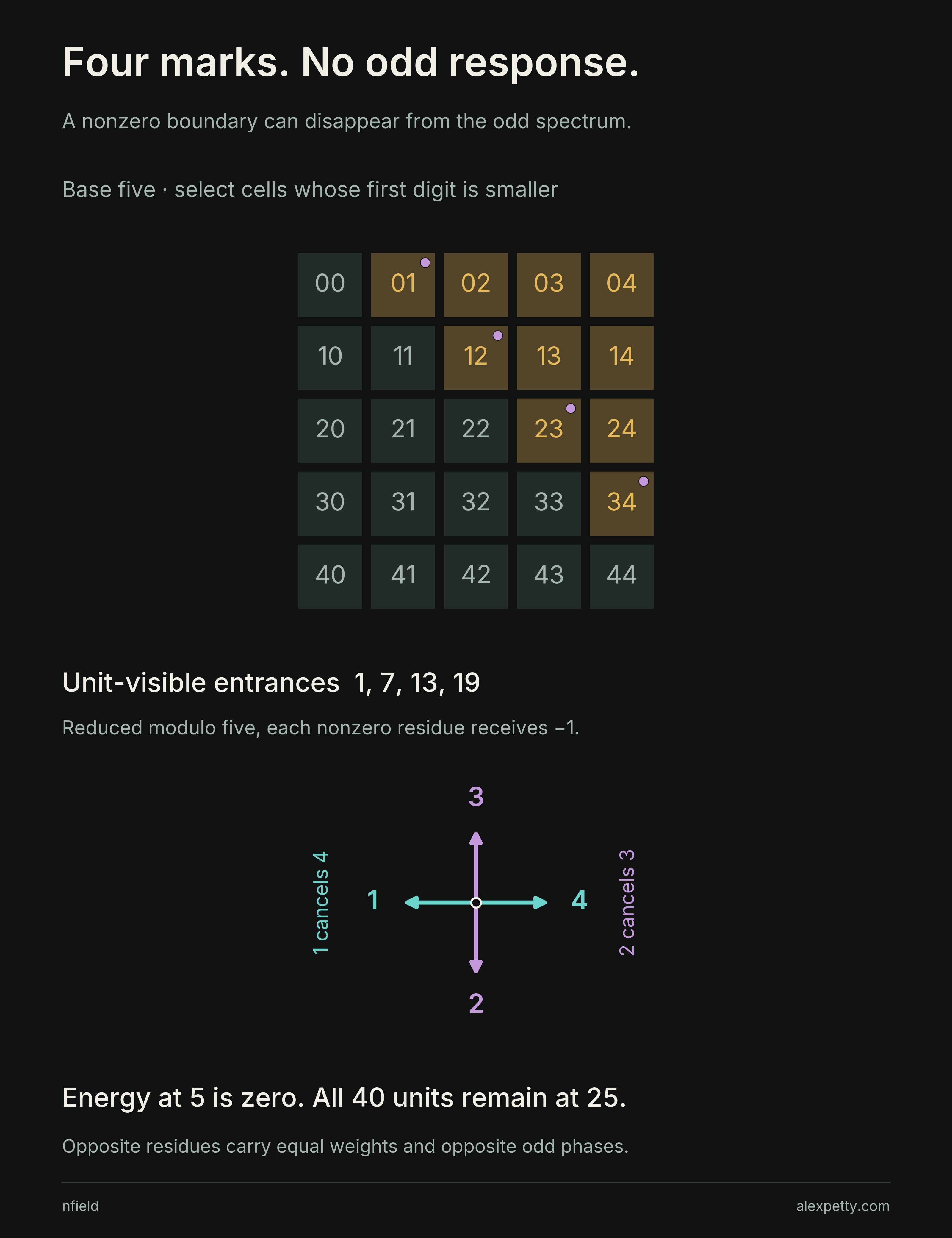
The collected boundary has not vanished. Its odd response has. Here $P_5=0$ and $P_{25}=40$.

For a general ledger, let

$$\begin{aligned} \Delta_d&=\sum_{r\in U_d}|M_d(r)|^2,\\ A_d&=\sum_{r\in U_d}M_d(r)\overline{M_d(-r)}. \end{aligned}$$

Odd-character orthogonality gives the energy through level $d$ as $\varphi(d)(\Delta_d-A_d)/2$. Isolate exact conductor $D$ by Möbius inversion,

$$P_D=\frac12\sum_{d\mid D}\mu_{\rm Mob}(D/d)\varphi(d)(\Delta_d-A_d).$$

The terms used to calculate $P_D$ can have signs. The resulting $P_D$ cannot be negative. Concentration at the top means every proper-conductor entry is zero. The exact condition at each level is that its primitive odd projection vanishes, which can happen while the collected boundary itself is nonzero.

The neighbor at minus one

The orbit is built by multiplication, yet its edge compares a remainder with its neighbor. Classical Jacobi sums describe exactly that meeting of the two operations.

For the orbit of squares modulo a prime, the calculation lands on a small and unexpected address. After the characters that are constant on the orbit are set aside, the remaining energy follows one of four formulas, chosen by the prime modulo eight. The proof explains the eight. Odd-character cancellation leaves a single contribution where the shifted neighbor is minus one, so the remainder itself is minus two. Whether minus two is a square is decided by the prime modulo eight.

The Jacobi calculation, including the endpoint correction

Let $q$ be an odd prime and $\psi$ its quadratic character. For an odd character $\chi$ not constant on the square orbit, define

$$J_+(\psi,\chi)=\sum_{y\bmod q}\psi(y)\chi(y+1).$$

The orbit flux is

$$S_H(\chi)=\frac{J_+(\psi,\chi)-1}{2}.$$

The minus one comes from the missing unit at zero. Indeed, extending characters by zero there,

$$\mathbf1_H=\frac{1+\psi}{2}-\frac{\delta_0}{2}.$$

Taking its additive boundary introduces $-(\delta_1-\delta_0)/2$. Pairing with $\chi$ contributes $-1/2$. The other unshifted character product sums to zero because $\chi$ is off resonance. That leaves the displayed formula.

The classical Jacobi magnitude is $|J_+|^2=q$. On summing over the off-resonant odd characters, orthogonality tests $y+1=1$ and $y+1=-1$. The first gives $y=0$, where $\psi$ is zero. The second gives $\psi(-2)$. Write $r=q\bmod8$. The supplementary laws for $\psi(-1)$ and $\psi(2)$ then yield

$$\begin{gathered} \mathcal E^{\rm off}(q)=\\ \begin{cases} (q-1)(q+3)/8,&r=1,\\ (q-3)(q+3)/8,&r=3,\\ (q-1)^2/8,&r=5,\\ (q-5)(q+1)/8,&r=7. \end{cases} \end{gathered}$$

At $7,17,23,31$ these are $2,40,54,104$. Off-resonant energy excludes any odd character constant on the orbit. At seven, the quadratic character is one such character. Its squared response is sixteen, making the full odd energy eighteen rather than two.

Jacobi sums and the study of neighboring power residues are classical. Lehmer, Lehmer and Mills study consecutive power residues, and Girstmair connects digit variance with Dedekind sums. The calculation here applies that arithmetic to the signed edge and separates its squared responses by exact conductor.

Additive Boundaries and Conductor Energies of Periodic Remainder Orbits gives the proofs, the expansion for higher-index orbits and the conditions under which a finite-state digit rule extends to a boundary on all residues. Its energy is measured before the Bernoulli factor. For primitive odd characters, multiplying the boundary response by the negative Bernoulli factor gives the carry coefficient.

Three compact views of the calculations

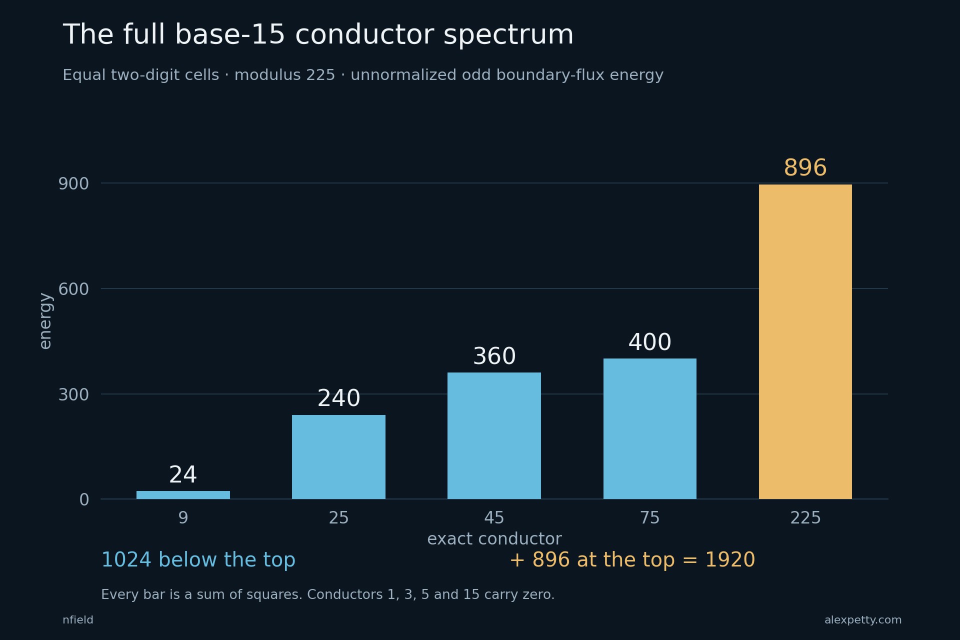
Back at $243$, the doubling circuit takes $162$ steps to come home, one for each remainder it visits. Its edge is the three-place pattern, an exit at a multiple of three and an entrance one step later, eighty-one times around the circle. The odd characters see those $81$ entrances all pointing the same way at conductor three and nowhere else, and the energy is $6{,}561$, exactly $81^2$. The base-fifteen rule, with only thirty formal edges, needs five conductors to hold its $1{,}920$.