Boundaries
Carry Boundaries and Bernoulli Spectra
Pick any question about the first two digits of a fraction, whether they are equal, whether the second is larger, whether they spell one particular pair. Each looks like its own small counting problem with its own count to do. Over all the fractions with a given denominator, though, every one of them reduces to a small table of carries, and the spectrum of that table splits the same way each time. One factor comes from the floor function and is identical for every question. The other is a short list of places where the question switches from no to yes and back, and that list is all a question gets to choose.
The shared factor is a generalized Bernoulli number, the one inside the collision coefficients of The Collision Spectrum, and the floor’s response is classical. The new part is the reduction itself, from any finite digit rule to its edges, and an accounting of those edges by conductor. For words whose first and last digits agree in an odd prime base, the edges have a clean average, twice their number. Base fifteen breaks it, giving where the clean rule predicts , and the accounting finds the difference at two lower resolutions.
Four matches at eleven
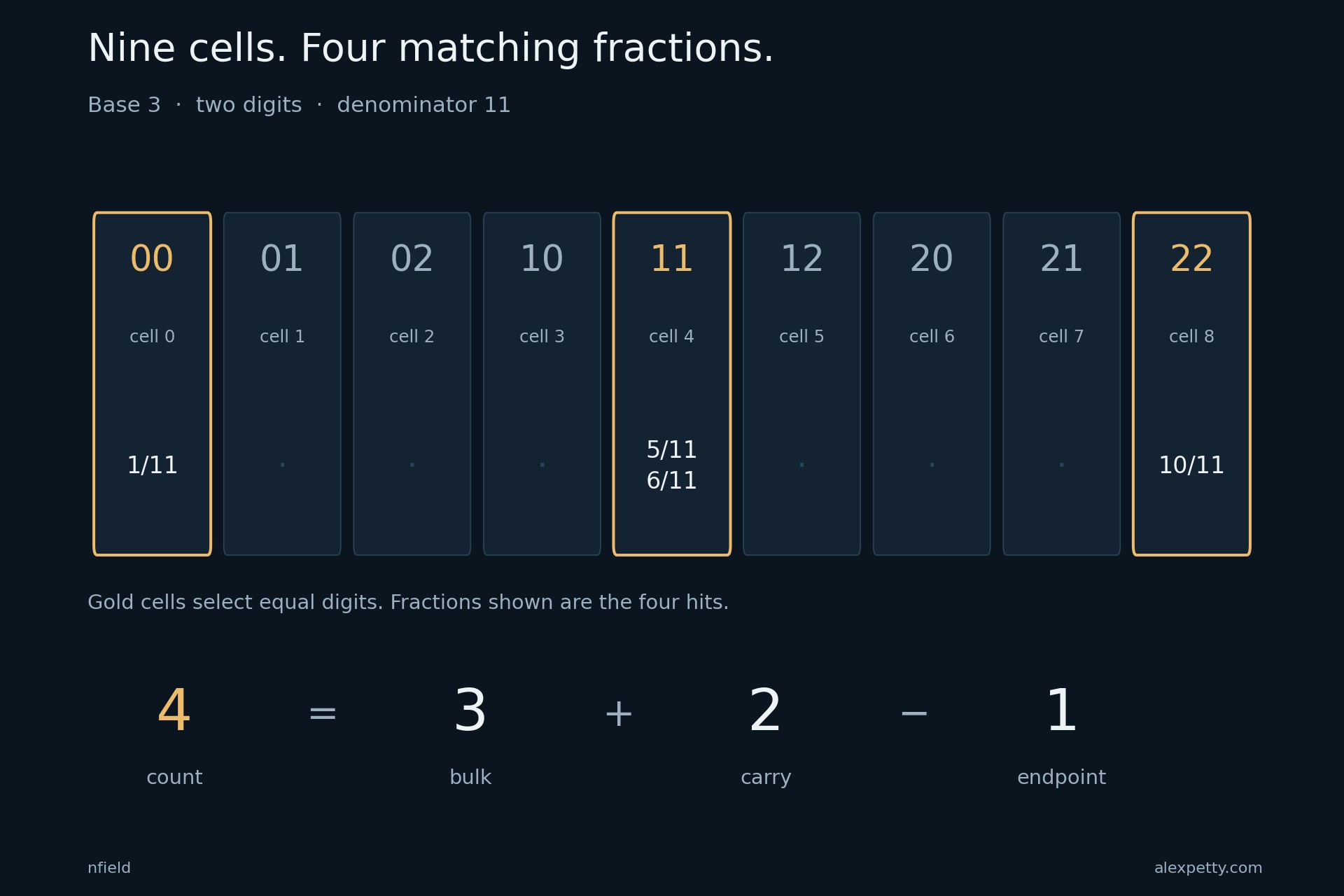
Base three keeps the example small. Divide each of through by eleven, in base three, and read the first two digits after the point. At numerators , , and they are , , and , four matches. The same count comes from a different picture. Split the unit interval into nine equal cells, one for each possible beginning in that order, and color the three cells with matching digits gold. A fraction passes the test exactly when it lands on gold. Any rule about the first two digits is a choice of cells, and the counting that follows works the same way for all of them.
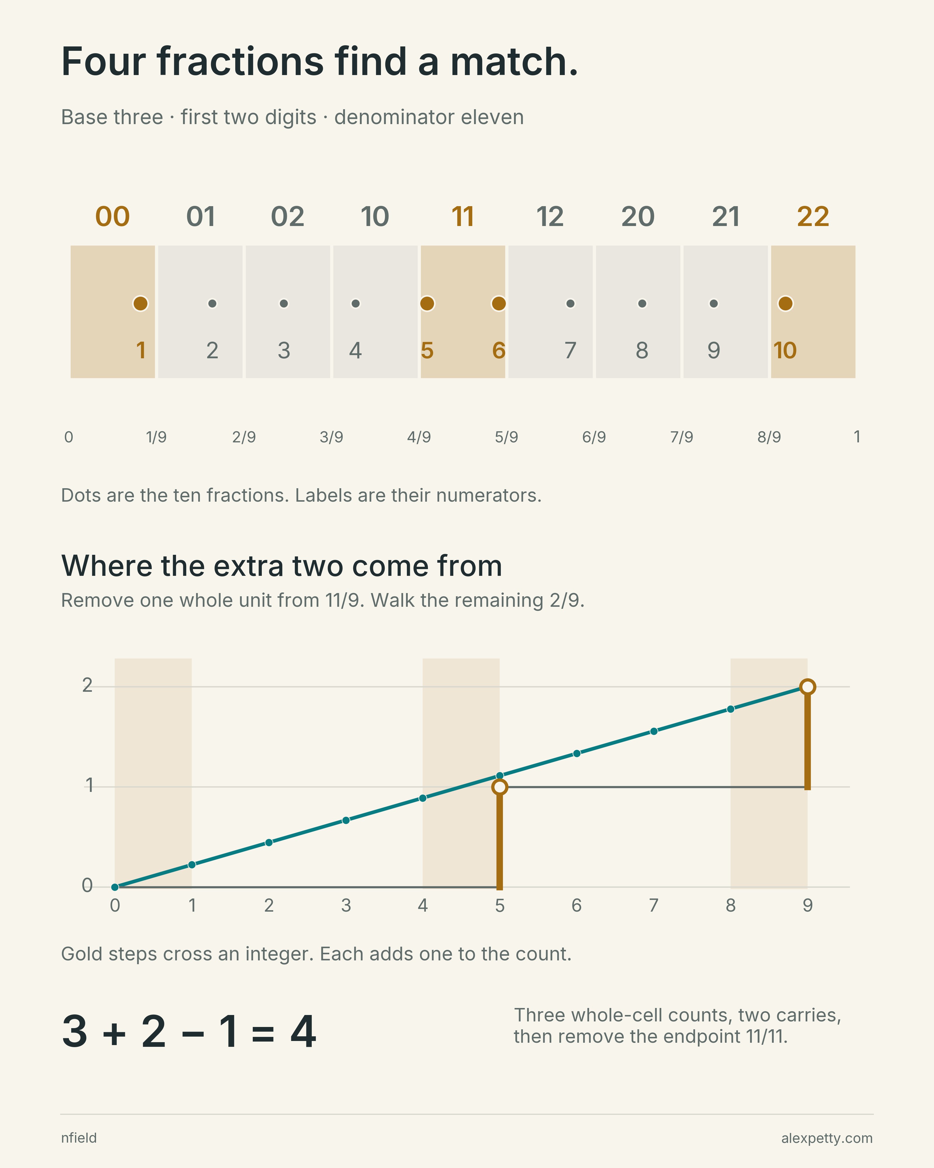
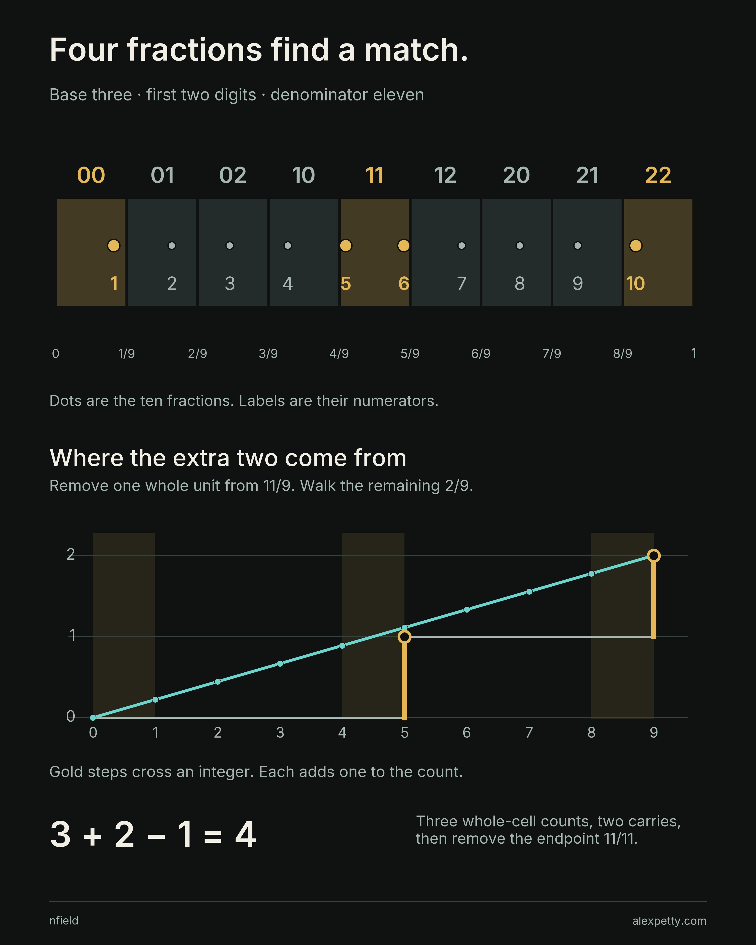
In the top row the ten fractions sit at their exact positions, and the gold cells , and catch numerators , , and . The cells are wide and the fractions apart, so some cells hold an extra fraction, and the extras can be counted without listing anything. Write as one plus . Each cell gets one whole fraction, and the leftover piles up from cell to cell. In the lower panel that running total is the teal line and its integer part is the staircase. The staircase rises twice, in cell at step five and in cell at step nine, and each rise is a carry that puts one more fraction in a cell. Both carries land in gold cells. Three gold cells give three whole fractions and the two carries give two more. The floor count also includes at the far end, though, while the fractions stop at . Removing it leaves
Replace eleven by twenty. Each cell now gets two whole fractions, but the leftover is still , so the carry walk is the same and the count is . Every denominator that leaves remainder two on division by nine reuses this little walk.
The floor count for any fixed digit rule
For a prefix of length in base , put . A weight records the rule on cell . It can be zero or one, or a more general numerical weight. Assume the denominator is coprime to the base and write , with .
The exact identity is
where
Each floor difference counts integers in the corresponding right-closed interval. Coprimality prevents a fraction from landing on an interior cell boundary. The last interval includes , which accounts for the subtraction. It is an endpoint correction.
At , the selected cells are , and . At , the same appears. The growing denominator changes the bulk count while the carry calculation stays finite.
Rub out the interior lines
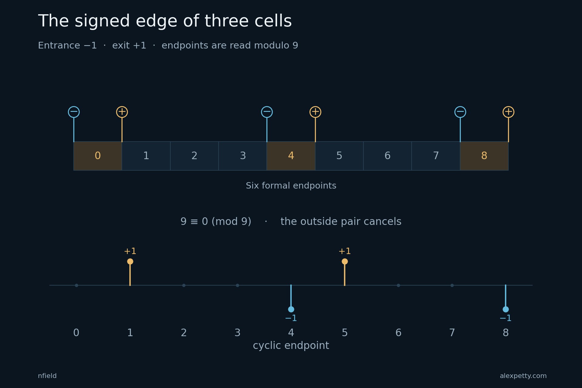
Now put two selected cells side by side. Each has an entrance and an exit, and at the shared edge an exit meets an entrance. Give them opposite signs and they cancel. A run of a thousand selected cells loses all its inside edges the same way and keeps only its entrance and its exit. The floor differences telescope in exactly this pattern.
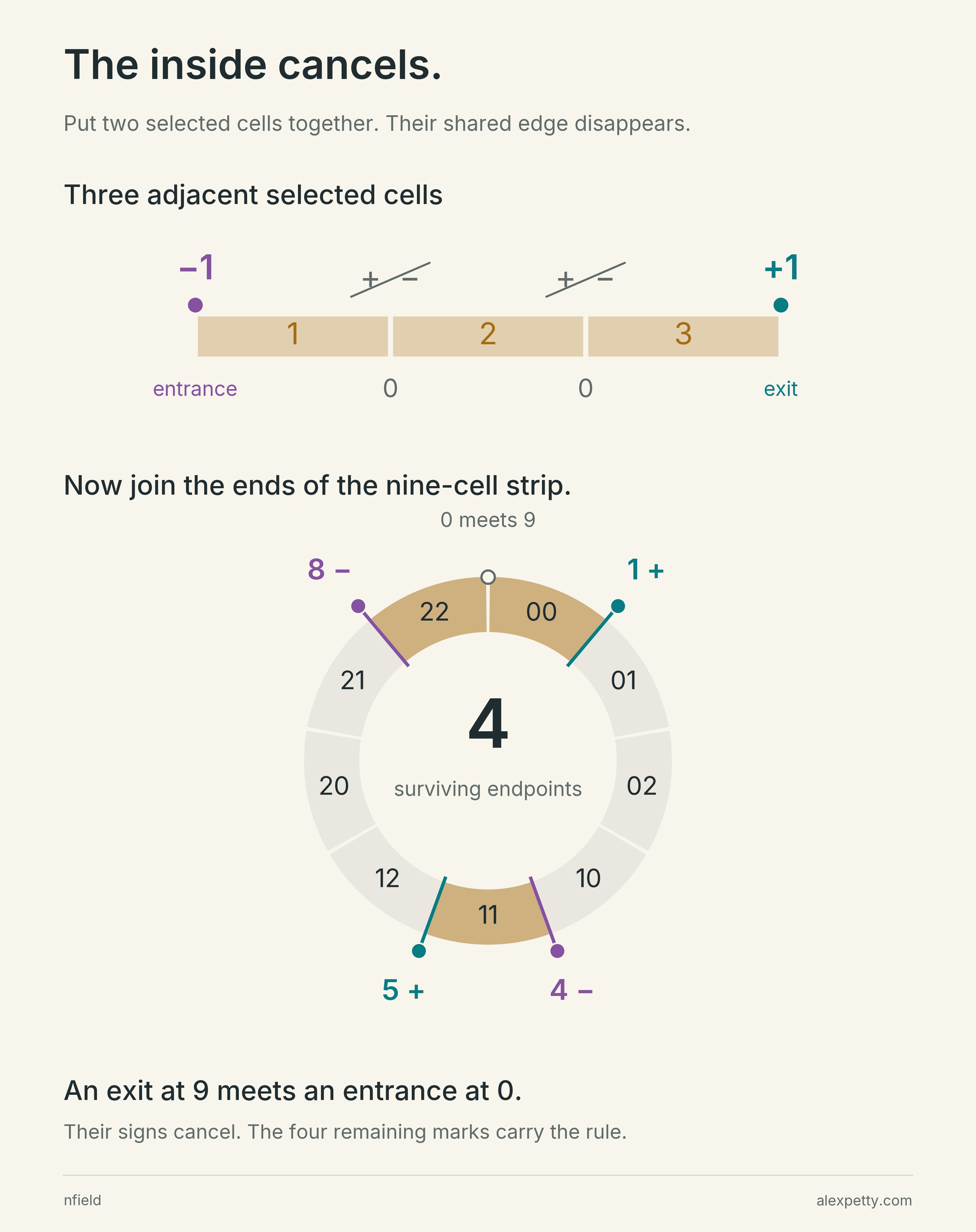
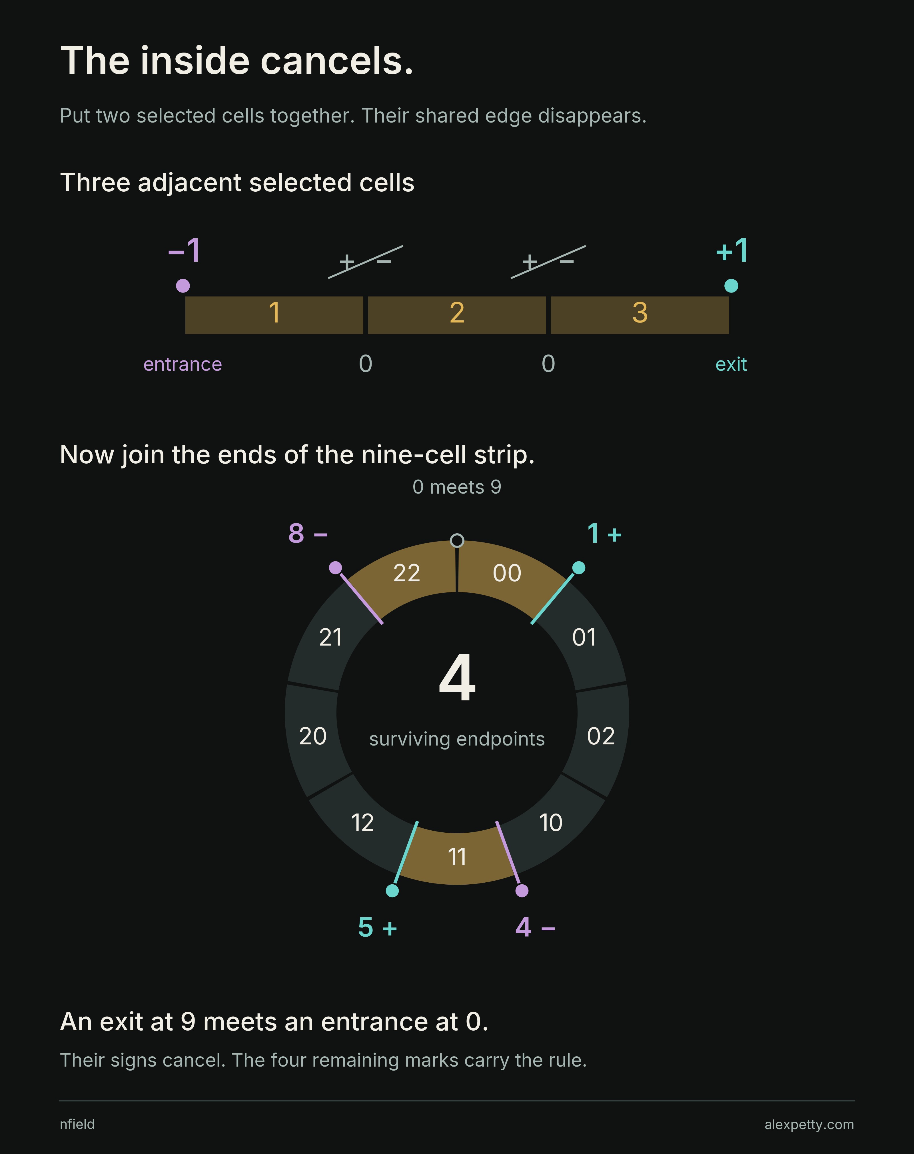
The upper drawing shows three selected cells in a row, with both inner edges cancelled and only the entrance at and the exit at left. The ring below closes the nine cells into a circle, so the exit after lands on the entrance at and those two cancel as well. Four signed marks survive, after , before , after and before . That boundary is all the rule leaves behind. Once the bulk count and the endpoint correction are removed, those four switches determine the whole carry table, and a long list of selected cells shrinks to a short list of changes.
The signed boundary and the sawtooth
With indices read cyclically, define
An entrance has sign and an exit . For the nonzero values are and .
The centered sawtooth is
extended periodically. Summing by parts gives the centered carry function
For unit residues , meaning , its relation to the floor count is
The last correction is zero for our example, because both end cells are selected. The complete six-entry table follows, with no interpolation between entries.
| Residue | Carry count | Centered value |
|---|---|---|
| 1 | 1 | 2/3 |
| 2 | 2 | 4/3 |
| 4 | 2 | 2/3 |
| 5 | 1 | -2/3 |
| 7 | 1 | -4/3 |
| 8 | 2 | -2/3 |
The sawtooth reverses sign under reflection, so . This is why its comparisons with even characters vanish.
Four arrows take the long way home
To read a spectrum, compare the carry table with arithmetic waves. A wave gives each allowed remainder an arrow, and multiplying remainders adds their angles. That is a Dirichlet character, drawn instead of written. The comparison can use every entry of the carry table, or it can start from the four signed endpoints alone.
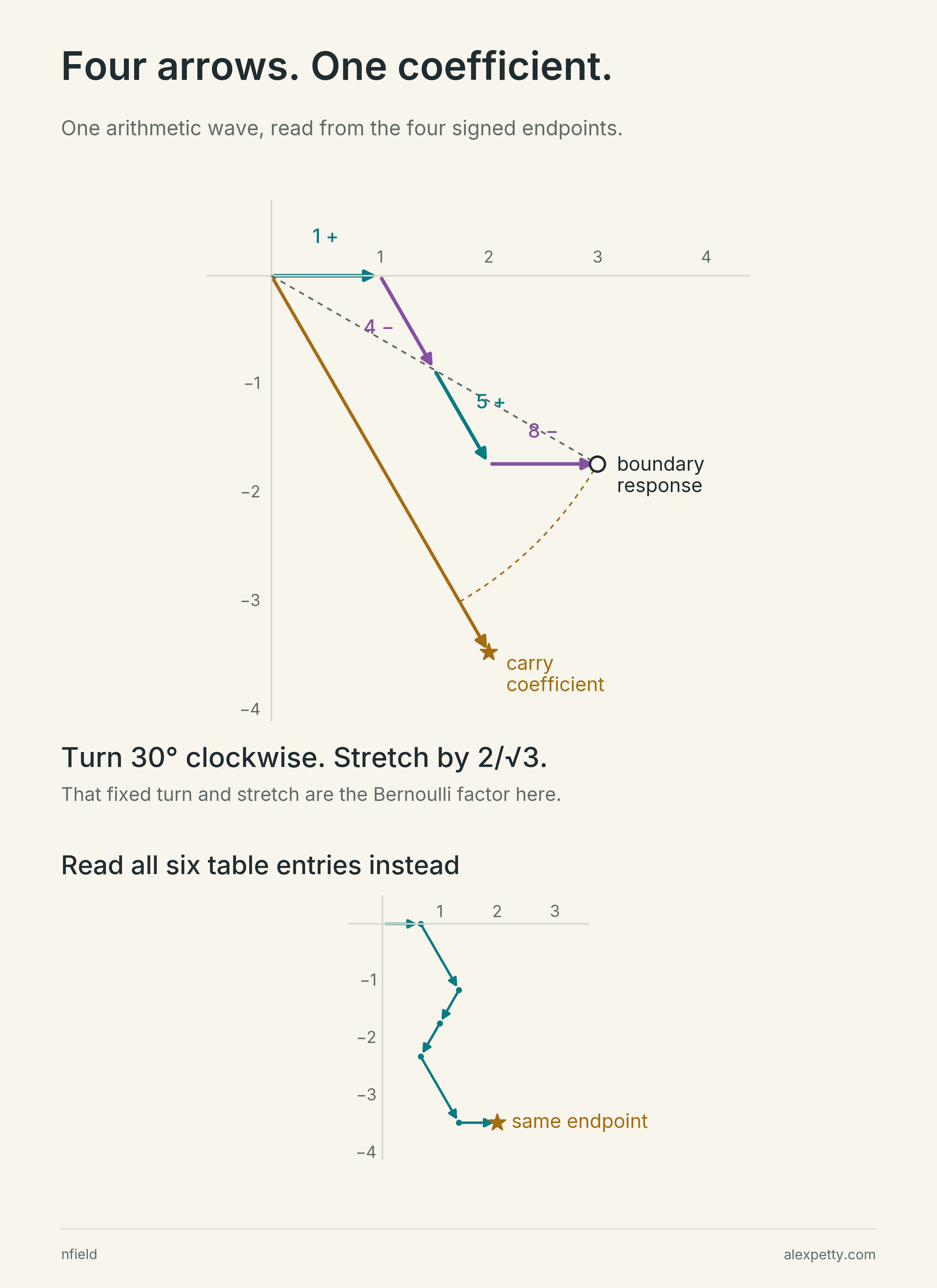
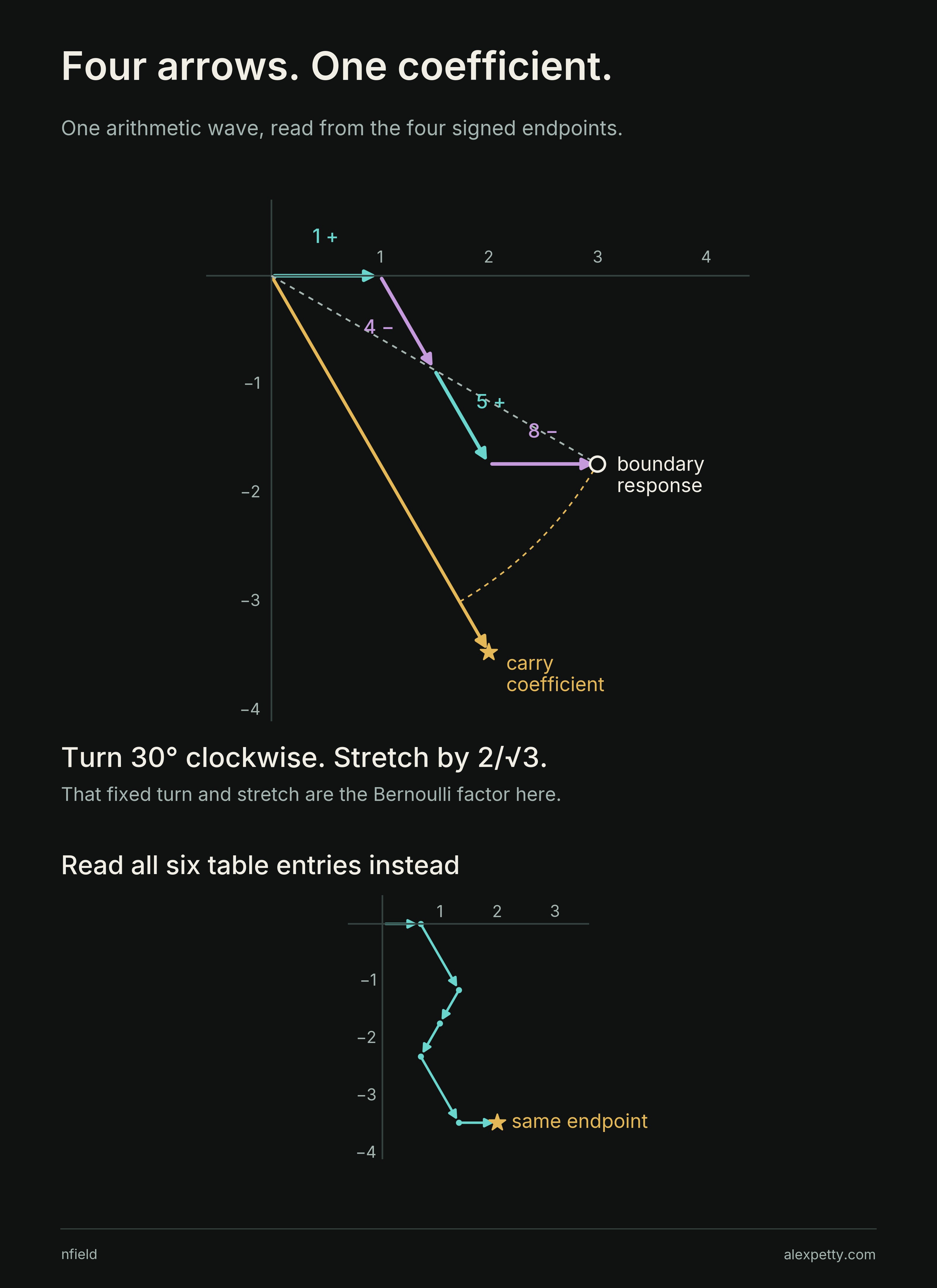
The upper drawing takes the second route, for the wave that turns sixty degrees at each doubling. Each endpoint contributes its arrow, reversed at an entrance, and the four arrows laid head to tail reach the open circle marked boundary response, at . Turning that point thirty degrees clockwise and stretching it by lands on the gold star. The lower drawing ignores the boundary and adds all six weighted carry values directly, and it arrives at the same star, .
The fixed turn and stretch come from the floor. Written as a complex number they are the negative of a generalized Bernoulli number, which enters because the fractional part climbs steadily between integers and drops back at each one, a sawtooth. For a primitive odd character, one that reverses under reflection and needs the full grid, that factor is the same whatever cells are colored. Change the gold cells and the boundary arrows change, while the floor keeps supplying the same turn and stretch.
The factorization and both routes to the gold star
A primitive character belongs to the full modulus rather than being inherited from a smaller one. An odd character satisfies . For such a character, define the ordinary boundary flux and the unnormalized carry transform by
Then the exact factorization is
where
For a unit endpoint , substituting in the sawtooth transform gives . For a nonunit endpoint, the primitive character sum vanishes. Applying this to the boundary sum proves the formula. Even coefficients vanish by reflection.
In the drawing, and . Multiplication by two visits and then returns to one. The arrow turns sixty degrees at each step.
The four boundary arrows sum to
The floor factor is
Its angle is minus thirty degrees and its length is . Multiplying gives
The lower path adds in the numerical order . It produces the same complex number. The conjugate character supplies the reflected coefficient. These are the only two nonzero coefficients of this table.
A finer grid can say nothing new
Split each of the nine cells into three, making twenty-seven, enough to read three digits, and keep all three children of each gold cell selected. The drawing is finer, but the test still asks only about the first two digits.
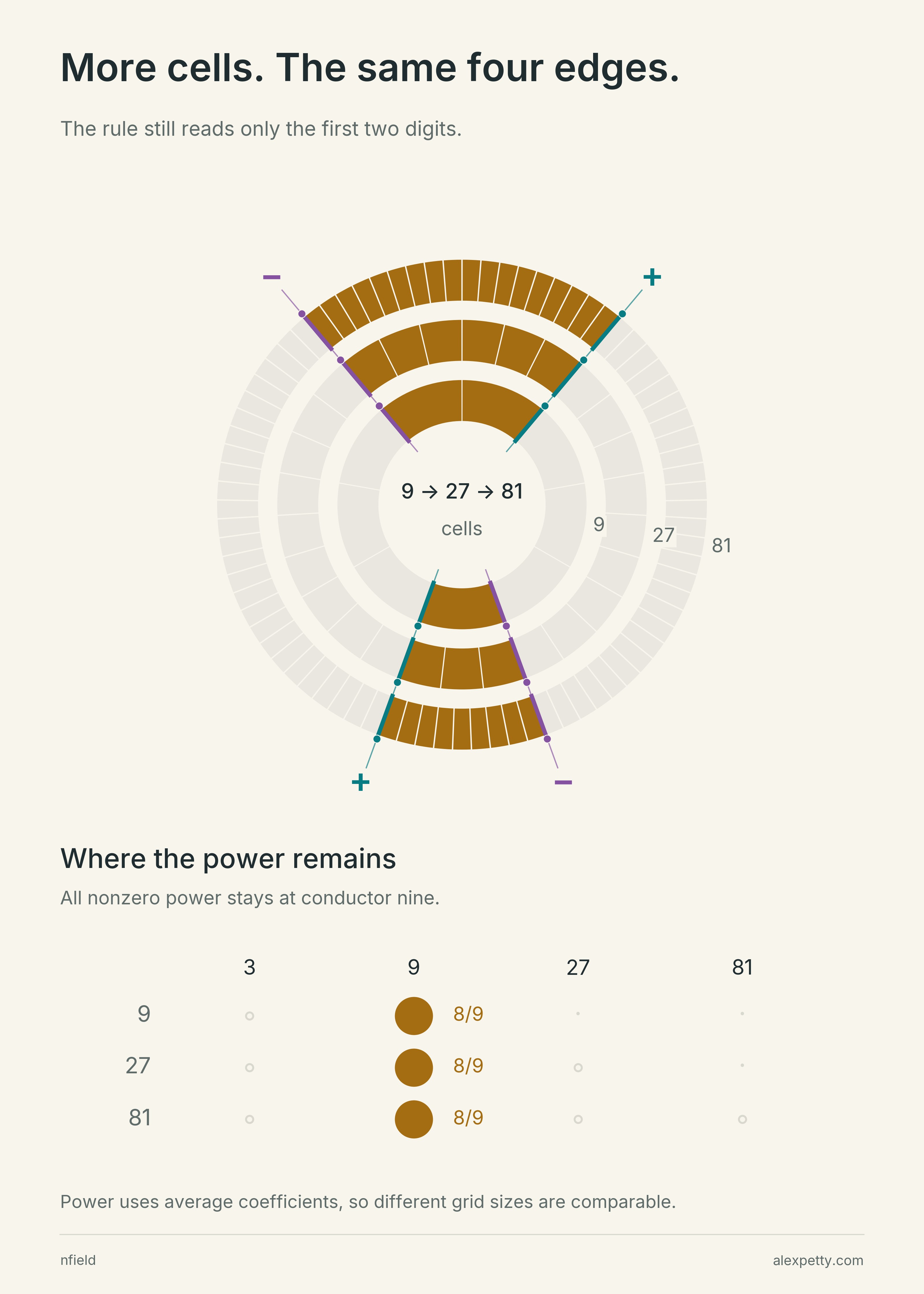
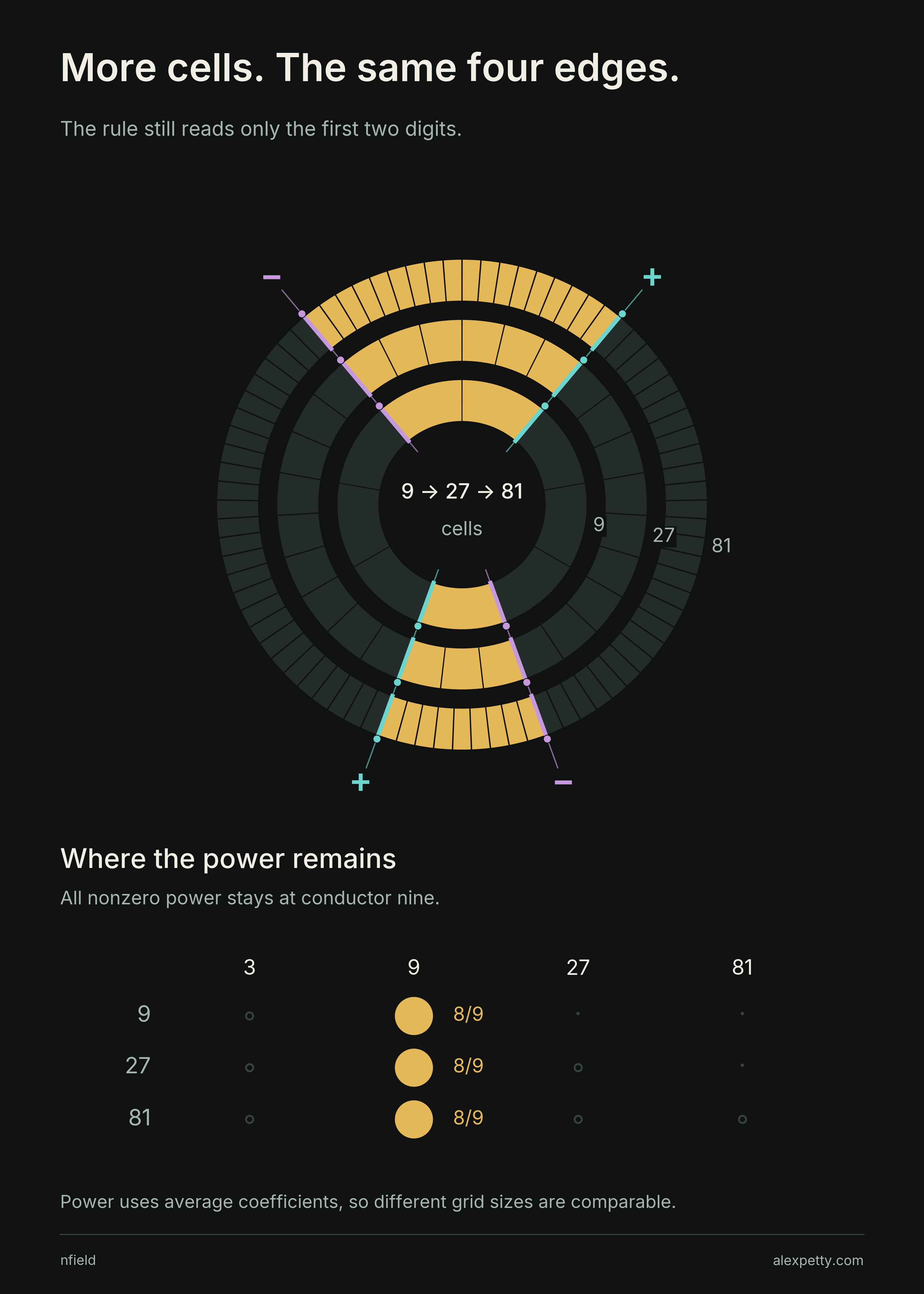
The rings in the figure go from nine cells to twenty-seven to eighty-one, and the gold arcs never move. Every new interior edge cancels, so the four border rays stay exactly where they were. The table below sorts the spectrum by conductor, the least modulus a character actually needs. Every grid puts its whole power, , at conductor nine, and the columns for twenty-seven and eighty-one stay empty. A finer grid that asks the same question adds no new response.
Refinement, and the limits of ordinary flux
At modulus twenty-seven the selected cells are
The surviving endpoints are , with signs . All are divisible by three, so every ordinary character flux modulo twenty-seven is zero. The primitive carry transforms are zero too, but the induced carry transforms need not be.
In fact . Each unit class modulo nine has three lifts. Thus an inherited unnormalized coefficient is three times its old value. The average coefficient, divided by the number of unit classes, is unchanged. The figure uses those average coefficients. Each of the two active characters has power , giving at conductor nine at every displayed resolution.
The distinction is essential. Ordinary fluxes determine exactly the boundary on units, because characters are zero on nonunits. They do not determine every induced carry transform. For a small counterexample, select cells zero and one modulo six. The two endpoints, zero and two, are nonunits. All ordinary fluxes vanish. Yet the odd character inherited from modulus three gives carry transform .
At a prime power , a character induced from a primitive character of conductor uses a depth-sensitive endpoint weight. For with ,
and the weight is zero at greater depth, including . The complete induced formula is
The additional weight recovers the information that ordinary flux discards.
Fifteen refuses the easy answer
The boundary also controls a clean average. In an odd prime base, select the words whose first and last digits agree, square the sizes of their primitive odd boundary responses and average them. The answer is twice the number of formal interval endpoints, counted before the cells are closed into a ring. The three gold cells in base three have six formal endpoints, and both primitive odd characters there give a squared response of exactly twelve.
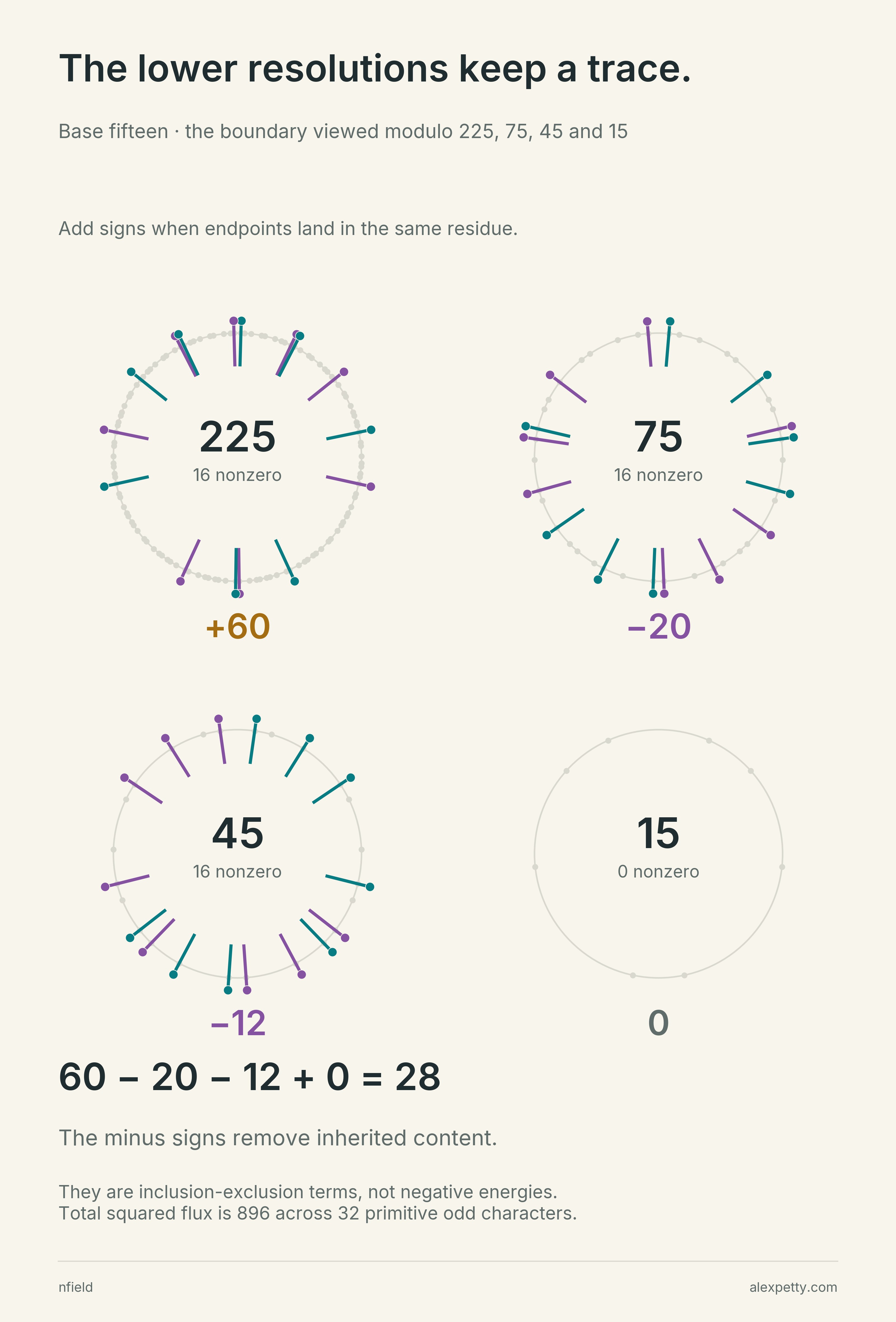
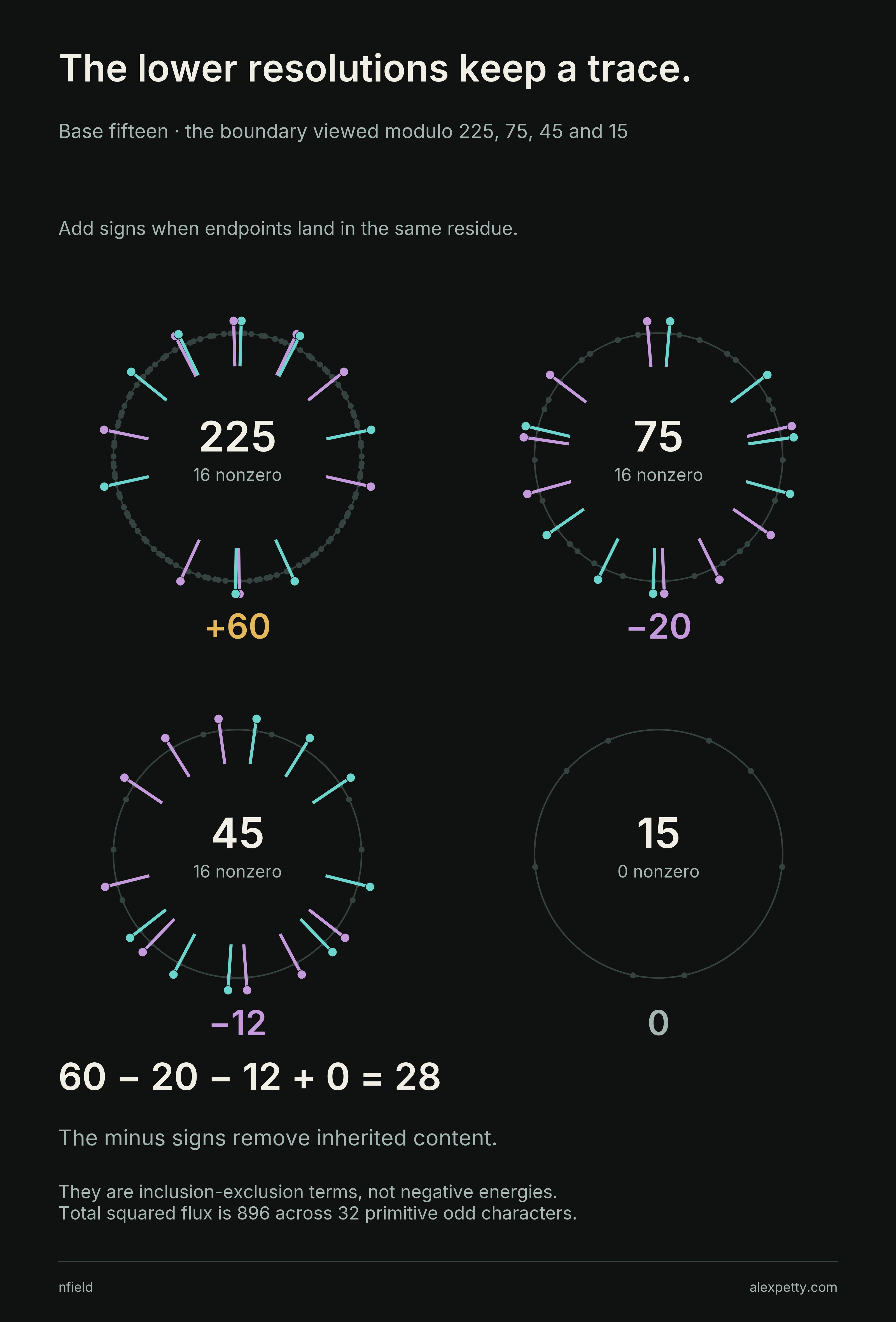
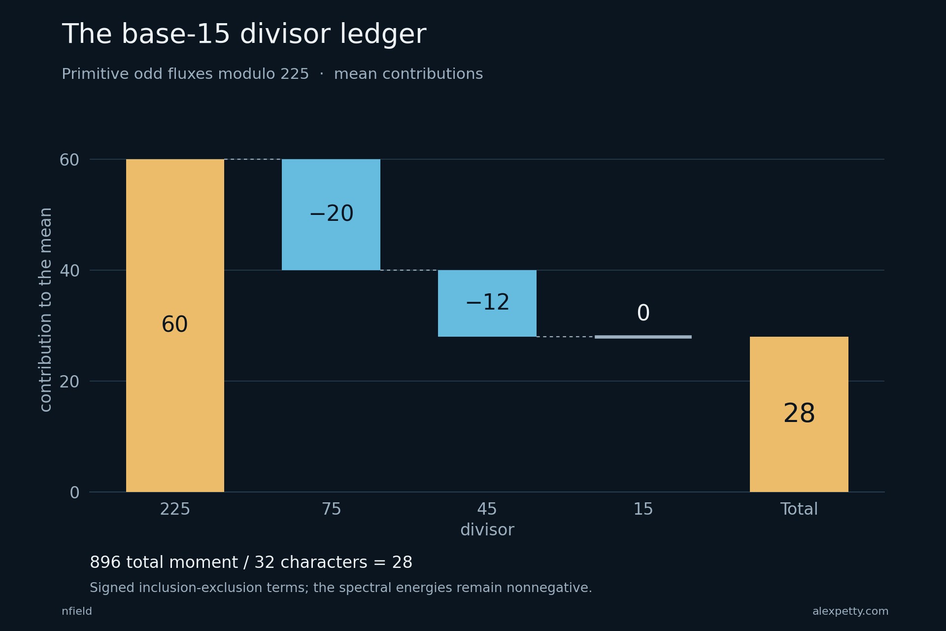
Base fifteen is where that rule fails. Its fifteen matching two-digit cells have thirty formal endpoints, which predicts , and the actual mean is . The missing can be located. Viewed modulo and modulo , the boundary still carries signed mass, and removing those inherited contributions subtracts and . In an odd prime base the corresponding lower sums cancel, and the clean answer depends on that cancellation.
See the surviving boundary at the lower resolutions
For an odd prime base and depth , the first-equals-last rule has formal endpoints. Its primitive odd mean is
Here . The proof uses two properties of the unit boundary. Reflection reverses its signs, and each unit residue class at the next lower resolution receives equal entrance and exit mass.
For a general modulus, restrict to units and collect its signed mass modulo each divisor . Write that collected mass as and set
The primitive odd total is given by the conductor ledger
The symbol denotes the Möbius function, not the signed boundary. Its signs perform inclusion-exclusion over conductors.
At base fifteen, and . There are sixteen nonzero unit-boundary entries. Their collected masses vanish modulo fifteen but not modulo forty-five or seventy-five. The only nonzero Möbius weights occur at the four divisors shown.
| Divisor | Squared norm | Reflection sum | Mean term |
|---|---|---|---|
| 225 | 16 | -16 | 60 |
| 75 | 16 | -16 | -20 |
| 45 | 16 | -16 | -12 |
| 15 | 0 | 0 | 0 |
The total is , across primitive odd characters. Dividing gives . Negative ledger terms remove overlap; the squared responses themselves are nonnegative.
Energy, Dedekind sums and the full proof
Adding the squared carry values defines an energy. Parseval gives its equivalent spectral expression,
The six values in our modulus-nine table give . On the spectral side, each of the two active coefficients has squared magnitude sixteen, so the same energy is .
Expanding the boundary formula gives a second description in terms of sawtooth correlations. At unit endpoint indices, these correlations are finite Möbius combinations of classical Dedekind sums. The Bernoulli factor on the character side satisfies
for primitive odd characters. Thus the finite carry energy retains both the selected boundary and classical arithmetic factors.
These are finite identities. Growth estimates as the base or depth increases require further bounds. A rule on a whole remainder orbit also needs more than the fixed-prefix boundary constructed here.
Carry Boundaries and Bernoulli Spectra in Long Division supplies the proofs, the general weighted formulation and the conductor-depth energy decomposition. Its archived editions retain the research record. The finite-table background is developed in The Collision Invariant and The Collision Spectrum.
Three compact views of the calculation
The question set aside at the start can be answered now. Ask instead whether the second base-three digit is larger than the first. The gold cells become , and , with edges at , , and . Two of those edges, and , are multiples of three, which no primitive character can see, and the two that remain are both entrances. Their arrows sum to , and the same thirty-degree turn and stretch by carry that to , exactly what the new carry table gives when it is added up directly.
That is minus half the collision coefficient, and for a reason. The equal, larger and smaller questions split the nine cells among themselves. Together they select everything, and a rule that selects everything has no edges and no spectrum, so their three tables add to zero. Reflection turns each fraction’s digits around and makes larger and smaller respond identically, which leaves each of them minus half of the collision table, , , , , and at the residues , , , , and .
Discussion
Sign in to join the discussion.