Collision Calculus

Refining a measurement is supposed to improve it. Read a curve at more and more evenly spaced points, average the readings, and the answer settles toward the area under the curve. The classical estimates for how fast it settles all share one assumption. They hold the curve still while the grid gets finer.

The arithmetic in this notebook will not grant that. Each finer grid arrives because the digit table underneath it has grown, and the field drawn over that table has grown along with it. The readings and the area can then stay a fixed distance apart however many readings are taken, and that gap is the quantity the proofs need.

That gap can be computed exactly, and the calculation is what Collision Calculus: Boundary Readings, Energy and Refinement is for. It starts with a line, three readings and two answers that are both correct.

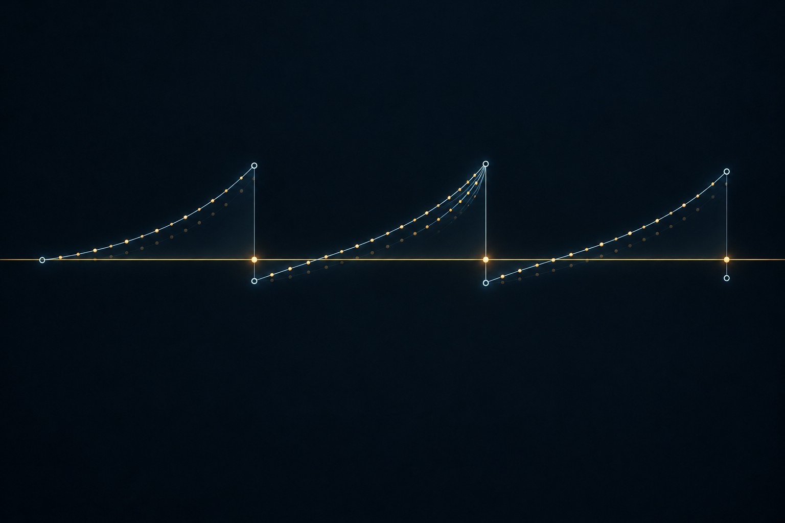
On the interval between zero and one, draw the line $f(x)=2x-1$. Repeat it. Each rising segment approaches one, then the next begins at minus one. At the reset itself, assign the reading zero, halfway between the two sides.

Now read the curve at zero, one third and two thirds. The readings are $0,-1/3,1/3$. Their squares average to $2/27$. The integral of the squared line is $1/3$, or $9/27$.

The difference is $7/27$.

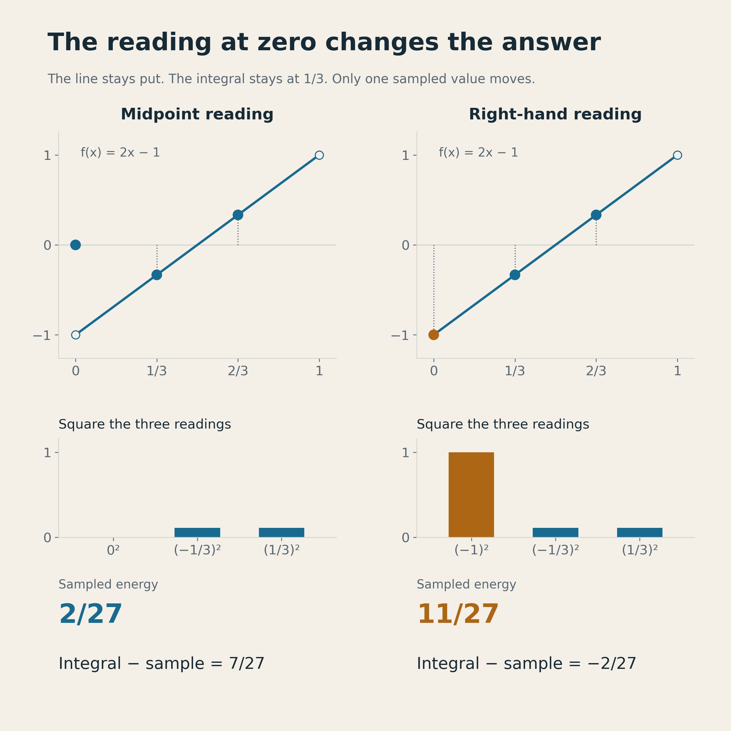
Change the reset reading to minus one. Nothing else moves. The sampled energy rises to $11/27$ and the difference becomes $-2/27$. The grid has gone from reading the continuous energy short to reading it long, on the strength of one dot.

The dot occupies no area. It has one third of the vote.

Four terms at a reset

I keep running into versions of this calculation. A finite digit table has a continuous description standing behind it. A carry resets several components at the same address. A finer observation admits new readings and changes the weight of the old ones. An estimate that was sound for one fixed curve can say very little about a family of curves that grows with the grid.

The individual tools are old and familiar. Euler-Maclaurin summation relates a sum to an integral. A squared norm records how two components interact when they are added before being squared. Summation by parts keeps the books when the weights change. What I have not found anywhere is their coordinated use on a specified field read by a specified observation, which is the work the word calculus does in the title. So I gathered that use into a text a reader can learn from without first going through the research notes that led to it.

The book teaches operations a reader can perform. Change a point reading. Combine two signals. Move the samples. Admit another clock. Keep the part of an infinite sum a finite computation has not reached.

The opening example shows why each of those operations needs its own accounting. Just before the reset the energy is one, and just after it, one again. At the reset the reading is zero. The sample carries weight $1/3$, so the missing square contributes $1/3$ to the difference.

That is $9/27$. The whole difference is $7/27$. The remaining terms owe $-2/27$, and tracking them down is the part of the calculation nobody gets to skip. A boundary contribution large enough to explain the answer can be opposed by what sits beside it.

The boundary formula in the book keeps four kinds of information. It records the readings at sampled boundaries, the jumps in the squared profile, the jumps in its slope, and the curvature along the pieces in between. Each of the four carries a weight that depends on where the grid falls. At the ramp’s reset the squared profile has no jump in value, since both sides approach one, but its slope changes sign. That slope term supplies the missing $-2/27$.

The four terms and what each one records

Put $h=|f|^2$. Use $q$ equally weighted samples at $(a+\theta)/q$, for $0\le a<q$. The offset $\theta$ is measured in grid cells, so $\theta=1/2$ moves every sample half a cell. The defect is

$$D_{q,\theta}[f]=\int_0^1 |f(x)|^2\,dx-\frac1q\sum_{a=0}^{q-1}\left|f\left(\frac{a+\theta}{q}\right)\right|^2.$$

For the piecewise twice continuously differentiable profiles treated in the book, Theorem 4.1 gives

$$\begin{aligned} D_{q,\theta}[f]={}&\frac1q\sum_{b\text{ sampled}}\bigl(\langle h\rangle_b-h(b)\bigr)\\ &-\frac1q\sum_b[h]_b\,\psi(qb-\theta)\\ &+\frac1{2q^2}\sum_b[h']_b\,\widetilde B_2(qb-\theta)\\ &+\frac1{2q^2}\int_0^1h''_{\rm reg}(x)\widetilde B_2(qx-\theta)\,dx. \end{aligned}$$

The brackets $[h]_b$ mean right trace minus left trace, and the angle brackets mean their average. The value $h(b)$ is a separate datum. The two periodic weights are the midpoint sawtooth $\psi(t)=\{t\}-1/2$, set to zero at the integers, and $\widetilde B_2(t)=\{t\}^2-\{t\}+1/6$.

For the opening ramp the point term is $1/3$, the value-jump term vanishes, the slope term is $-2/27$, and the regular-curvature integral vanishes. Changing the reset reading removes the point term and leaves the rest where it was.

Two pulses that cancel

Two signals of height one need not carry twice the energy of one. Add them in agreement and the height is two, whose square is four. Add them against each other and nothing is left standing. The separate squared heights come to two in both cases. The whole difference lies in their interaction, and for real readings that interaction is the middle term of

$$(f+g)^2=f^2+2fg+g^2.$$

Laying a second identical ramp on the first quadruples the three-reading defect, from $7/27$ to $28/27$. Adding the two defects separately gives $14/27$, exactly half the right answer.

A sharper example comes later in the book. Take two flat pulses, each of height two and width one half. Delay the second by one eighth and subtract it from the first. Most of the two pulses cancel, leaving a short positive piece at the left end of the interval and a short negative piece halfway across.

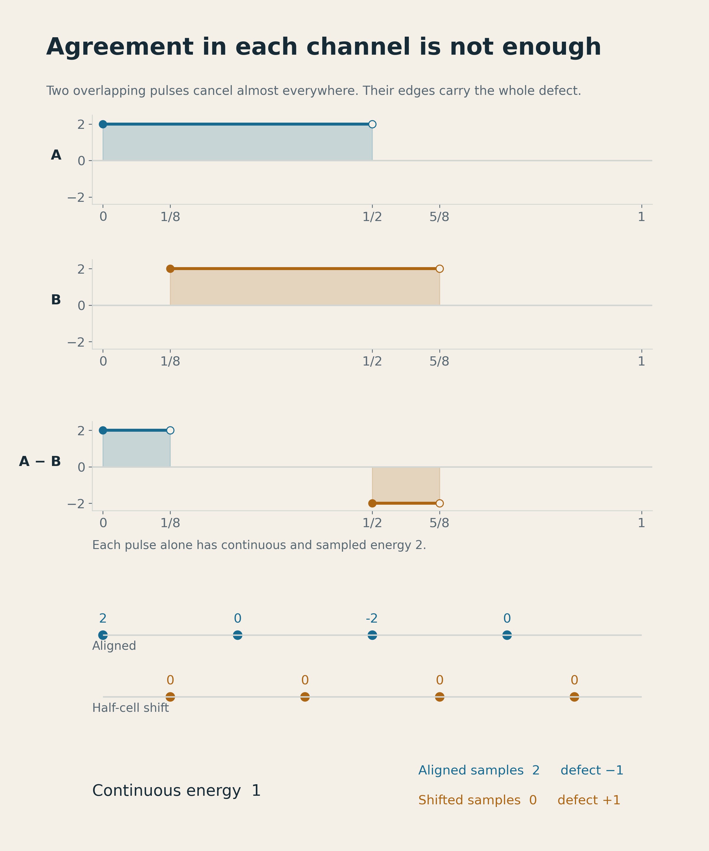
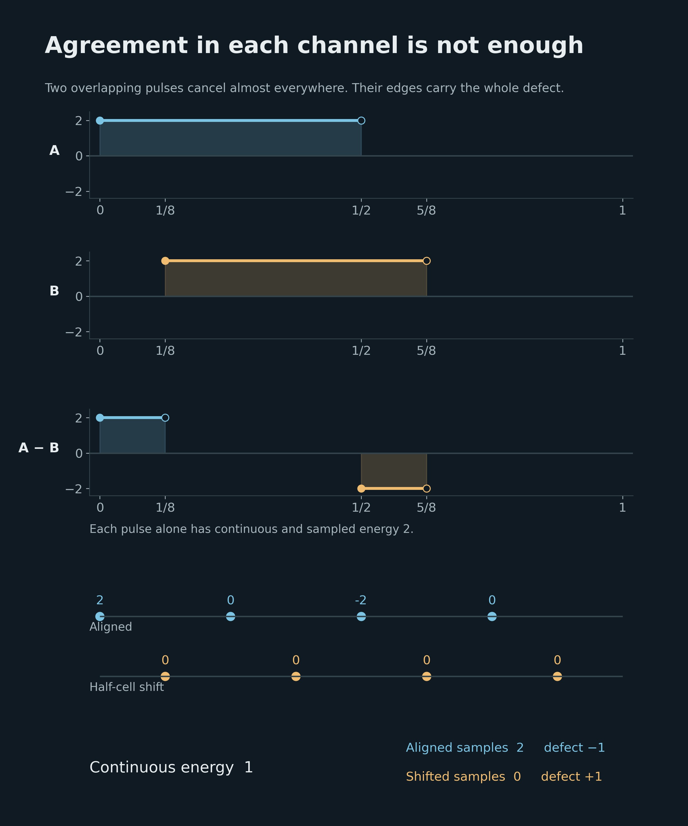
The continuous energy of that difference is one. Four aligned samples catch both surviving pieces and report an energy of two. Move the same four samples half a cell and they land where the difference is zero, so they report nothing at all.

Each pulse on its own is measured exactly by both grids. Their difference has defect minus one on the aligned grid and plus one on the shifted one, and every bit of it comes from the mixed term. That makes a good test to put to an energy calculation. Hand it two channels it measures exactly, then ask it for their difference.

A ramp that grows with the grid

More samples do repair the opening ramp, as long as the ramp holds still. With $q$ readings instead of three its defect is

$$D_q[f]=\frac1q-\frac{2}{3q^2},$$

which falls to zero like one over $q$. That is the behavior the textbooks promise.

Now let the ramp grow taller as the grid grows finer. Multiply its height by $\sqrt q$. Squaring multiplies both energies by $q$, so their difference becomes

$$D_q[\sqrt q\,f]=1-\frac{2}{3q}.$$

It climbs to one.

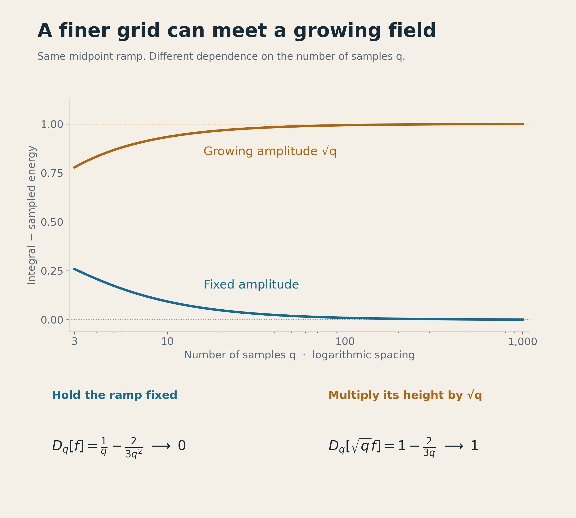
At a thousand readings the fixed ramp is off by just under a thousandth, and the growing ramp by just under a whole unit. Both experiments take the same thousand readings. Only one of them has been reading the same thing throughout.

The pulses can be made to grow this way too. On an even $q$-point grid, give them height $\sqrt q$ and separate their starting points by $1/(2q)$. Their difference then occupies two shrinking intervals, each of width $1/(2q)$ and squared height $q$, so the continuous energy stays one. Aligned readings report two and half-cell readings report zero. Those answers are exact at every even grid size, with no limit taken.

This is the distinction the research problems force. Their fields grow as their arithmetic tables grow, so a bound whose constant was fitted to the old field cannot be carried across to the next one.

One quarter, half a cell over

The clocks in the collision papers are rising, resetting waves. The first makes one turn around the interval, the second two, the third three. In prime base $p$ the carry field holds the first $p-1$ of them, and its natural grid has $p^2$ sample points.

At zero every clock resets together. The jumps combine before the square is taken, which is why the sampled point contribution is

$$\frac{(p-1)^2}{p^2},$$

a quantity that approaches one. The Common Reset in the Cubic Law follows that contribution and the signed estimate needed to prove the full defect approaches one as well.

Now move the grid half a cell. It no longer reads zero at all. It does read one half, where the clocks of even frequency reset, and there are exactly half as many of those.

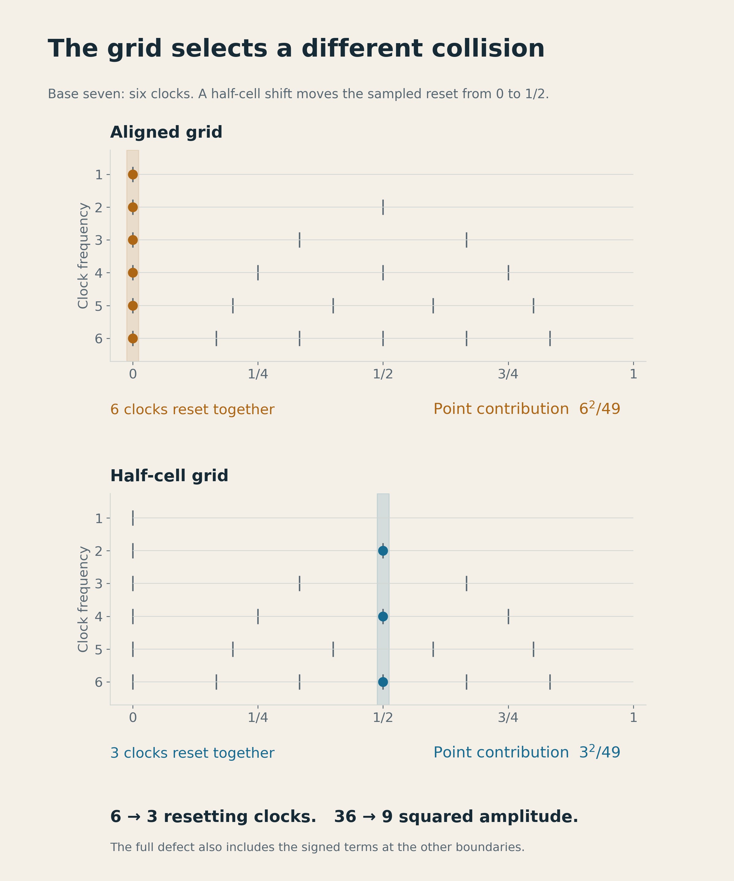
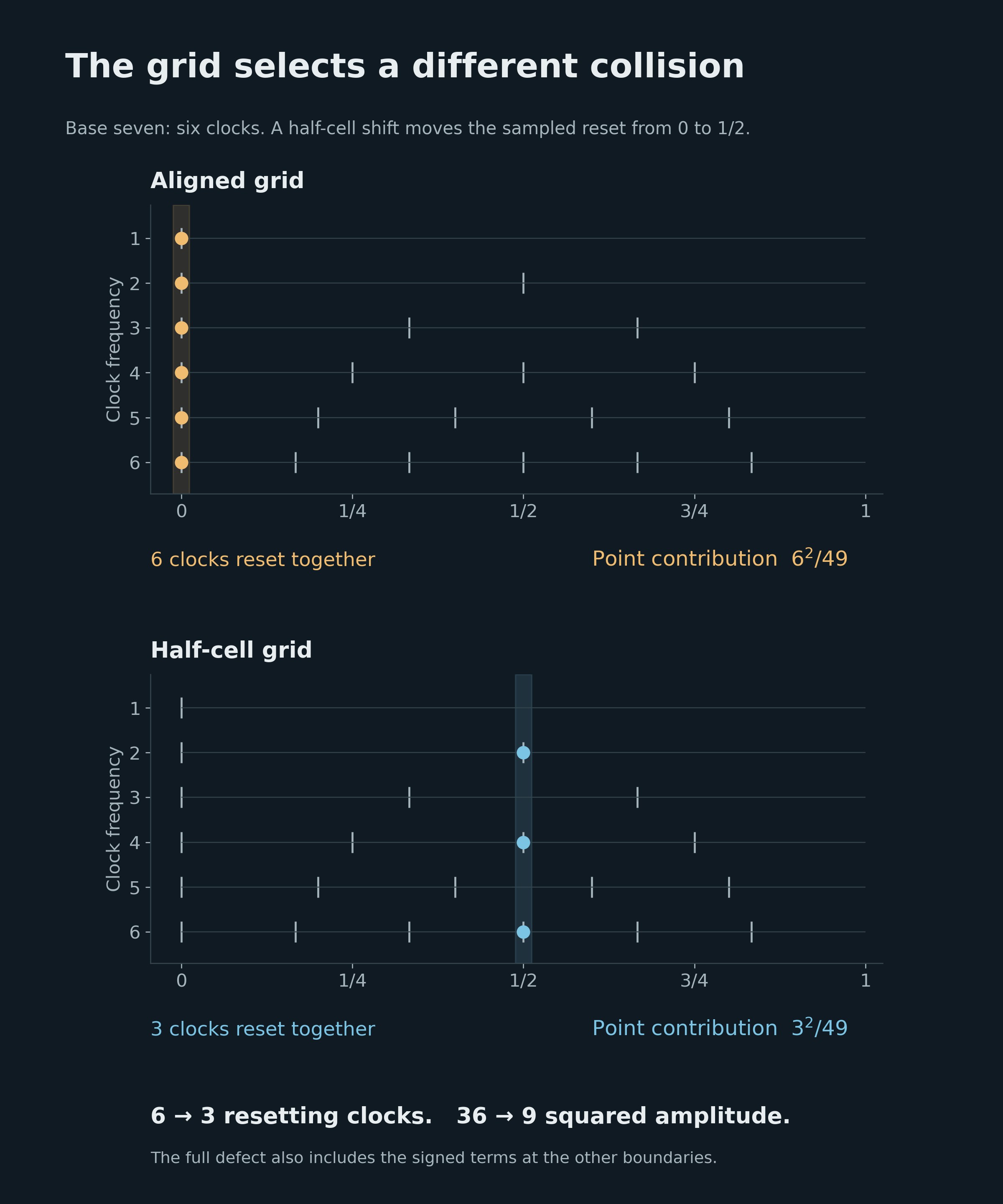
Half the combined amplitude gives a quarter of the squared amplitude, so the new point contribution is

$$\frac{(p-1)^2}{4p^2}.$$

One quarter becomes the candidate limit. Proving it is another job, since the unsampled boundaries contribute signed terms of their own and moving the grid changes those terms as well. The book carries the even and odd distinction through the arithmetic estimate and shows the remaining terms falling away. The shifted defect does tend to one quarter as $p$ runs through the odd primes. That half-cell limit is the book’s main new piece of arithmetic.

At small bases the remainder is plainly visible. At base 53 the shifted point contribution is about $0.240655$ while the full defect is $0.259267$. At base 97 the point contribution has risen to $0.244872$ and the full defect has fallen to $0.206508$. A boundary term can approach its limit smoothly while the answer around it goes on fluctuating.

The reset pattern at bases 7, 13, 31 and 97

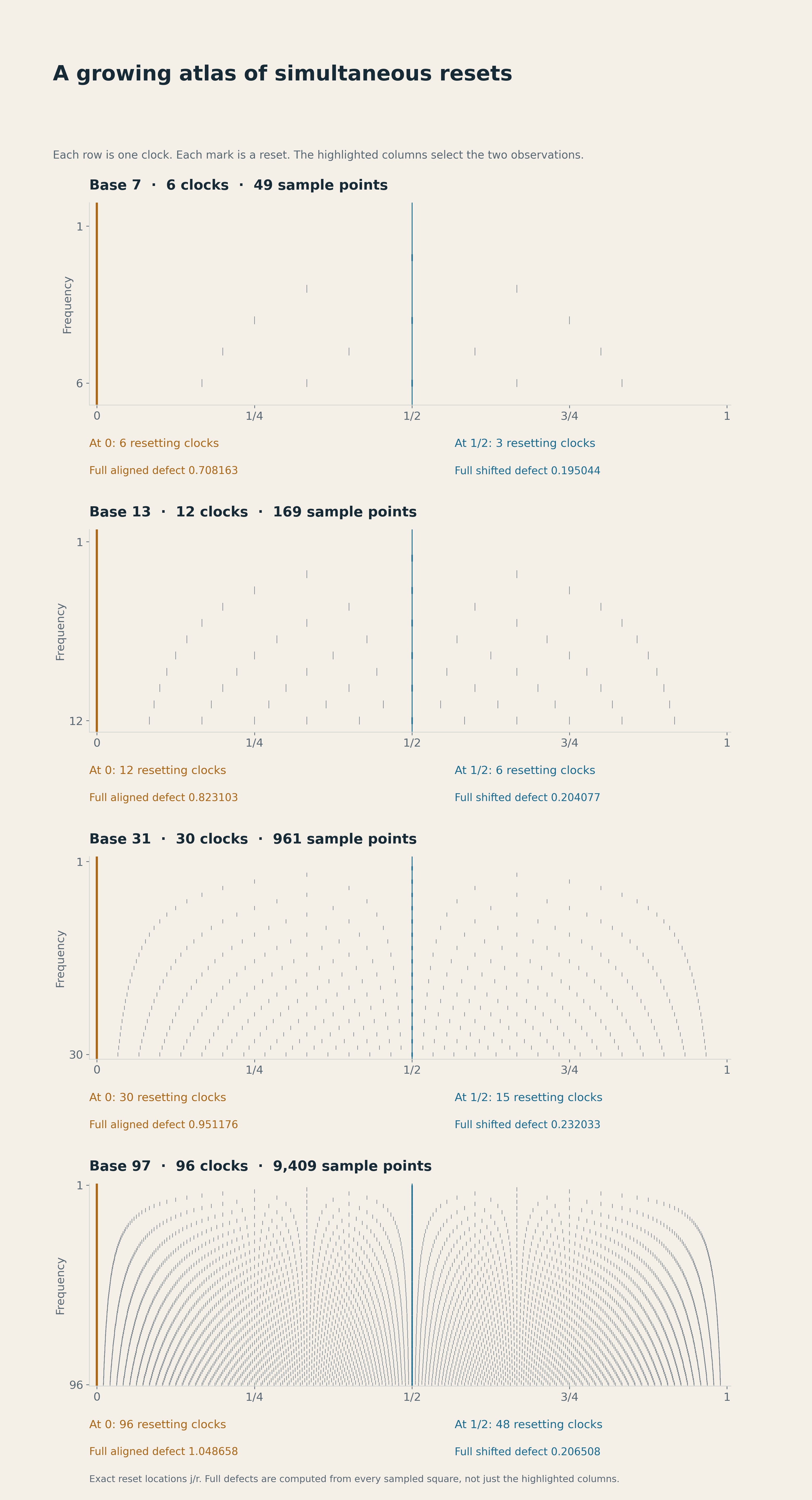
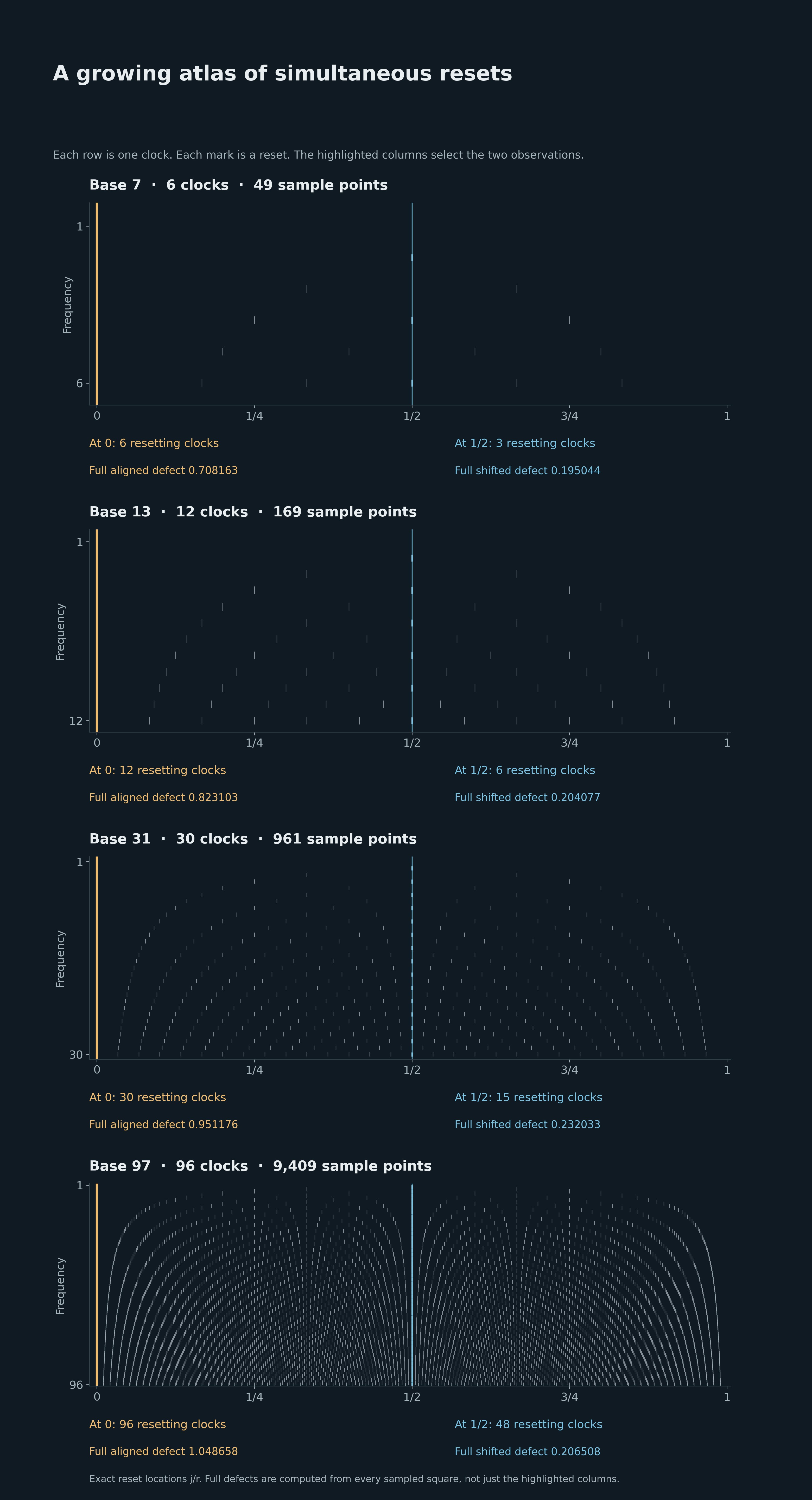
Every mark is an actual reset at a fraction $j/r$. Vertical alignments collect the clocks whose periods meet at the same address. All the rows align at zero. Every other row aligns at one half. The counts grow with the base and that ratio holds.

The full defects drawn under each panel are computed independently, from the sample squares and the continuous pairwise energy, so they include the signed remainder. These four examples illustrate the calculation. The limit rests on the estimate in the book rather than on a visual trend.

A bend no line can remove

The book also asks a question from the other direction. Suppose a field can be corrected, but only by additions of a restricted kind. How much of its energy has to survive the correction?

Take three readings, $(0,1,0)$, each with weight one, and allow any straight line to be added to them. The line can raise the readings, lower them or tilt them. It cannot take out their bend.

Measure the bend by taking the first reading, subtracting twice the middle one, then adding the last. For these readings the result is minus two. For any straight line it is zero. So minus two survives every correction the rules allow.

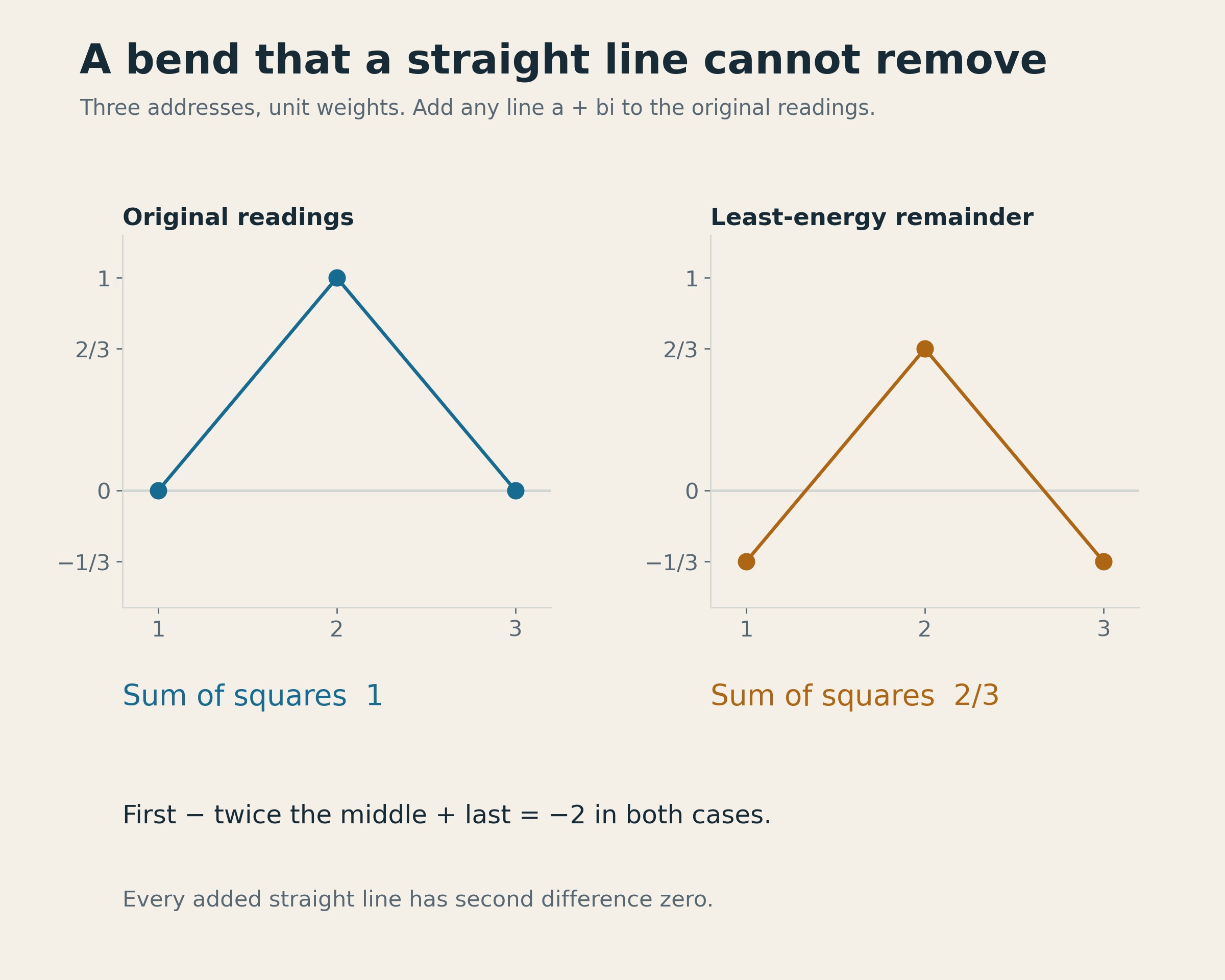
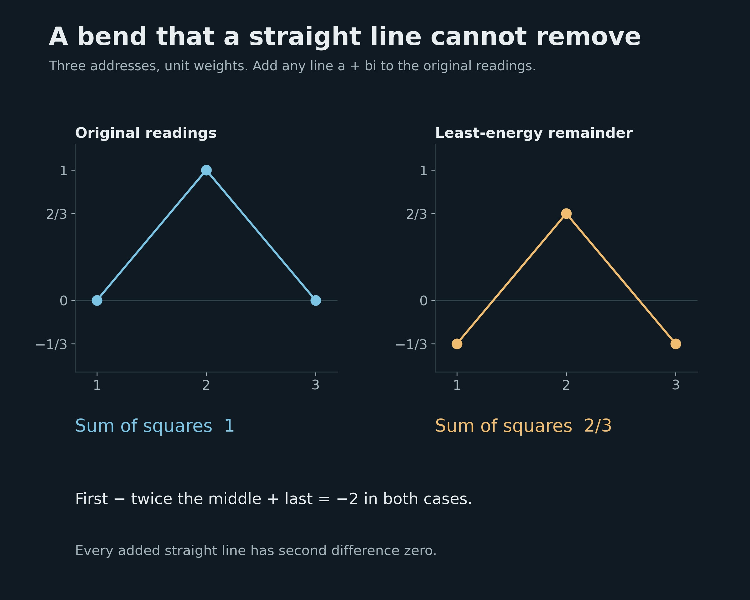
Subtract one third at all three addresses and the readings become $(-1/3,2/3,-1/3)$, whose squares sum to $2/3$. No straight-line correction does better. The book takes the lower bound from Cauchy-Schwarz and then exhibits this correction attaining it.

With more addresses there can be several surviving combinations at once. If they overlap, their separate lower bounds cannot be added together, since that would charge twice for the same retained energy. A matrix records the overlap and returns the joint cost.

Least squares and linear constraints are old mathematics, and I put them to one practical use. Before hunting for a better arithmetic approximation, find a reading that none of the permitted corrections can touch. Whatever energy that reading holds, the hunt is not going to recover it.

Weights that reach every address

Some of the later observations run over every positive integer. The weight at address $n$ is

$$w_n=\frac1{n(n+1)}=\frac1n-\frac1{n+1}.$$

The first address carries half of the total mass and the second a sixth, which leaves a third for everything from the third address onward. Resolve one more address and that third splits into a twelfth and a quarter. The total is one throughout.

The constant field one gives a fixed target to aim at through all these subdivisions. Its energy stays one. A more detailed description of it has not created any more energy, and the new readings, or the new fields brought in to approximate it, need their own accounting.

A sum that stops at address $N$ still owes an account of everything past it. The observation mass out there is exactly $1/(N+1)$. If the old and new fields have heights bounded by $A$ and $C$ beyond that address, the omitted change in energy lies between $-A^2/(N+1)$ and $C^2/(N+1)$. That interval belongs beside the finite answer wherever the finite answer is quoted.

The book works a two-clock example where the danger is easy to see. Stopping at address four gives an energy change of $-1/4$. The complete change is $3\log2-2$, about $+0.07944$. Restoring the tail reverses the sign.

Working through the book

The opening part develops boundary readings with lines, resets and pulses. The next part changes the fields and the rules for observing them, taking in overlapping corrections and moving weighted windows. Finite arithmetic enters after that, through congruences, collision registers and divisor sums. The last part returns to carry grids and growing clock families, where the method has to face the estimates that called for it.

The early calculations need calculus, finite sums and elementary linear algebra. Fourier series come in with the proof of the boundary formula. The later arithmetic asks for more. Worked examples sit next to the operations they teach, and the independent problems have hints and solutions at the back. A glossary and subject index give a way back to a definition without rereading the argument.

I have kept the unfinished work in plain sight. The half-cell carry limit is proved. A uniform estimate for the signed change in the native divisor-field energy is open, and the book preserves the full expression that needs bounding, including the old field’s contribution and the infinite tail. A finite calculation can inspect that expression at any one size. Certifying every size is the work that remains.

The book is available here. It collects a method I keep needing, puts it in an order that can be taught, and returns the reader to the calculations where it has work left to do.

Return to the first graph. The line has not moved. With the dot at zero the grid reads $2/27$ against the integral’s $9/27$, and with the dot at minus one it reads $11/27$. The integral cannot tell those two fields apart. Both of the grid’s answers are exact.