The Common Reset in the Cubic Law

Redefine a function at a single point and its integral stays exactly where it was. A list of samples is less forgiving. Change one of twenty-five readings and the average moves by a twenty-fifth of the change. Usually that does no harm, because each sample’s share shrinks as the grid gets finer and the sampled average settles onto the integral. That shrinking share is the reason a fine enough grid can stand in for an integral at all. The carry table behind digit-collision energy is that kind of grid, and it holds one sample whose effect never shrinks away.

The table gets finer as the base climbs, and the curve it samples grows along with it. That curve is a sum of sawtooth clocks, one more clock for every step up in base, and at zero every one of them resets at the same moment. On either side of zero the clocks agree, and their sum nears the largest size it can have, while at zero itself the table records a reading of zero. At base 1,009 that reading is one of 1,018,081, and correcting it alone would still move the average by 0.998. As the base grows, that correction approaches one exactly.

The Secondary Term of the Cubic Law leaves this difference between the table and its curve unresolved. Every table it computes points to one, but its proof can only keep the difference below a bound that grows with the base. The paper behind this article proves the limit is one, and that the reset at zero accounts for all of it. The other resets, all 308,925 of them at base 1,009, leave a combined remainder there of 0.039, and the paper proves that remainder tends to zero.

Most of the tools are classical. Dedekind sums and their reciprocity law, Weil’s bound for Kloosterman sums and the derivative estimates for exponential sums all have long histories. The new parts are an exact identity that separates the reset at zero from everything else, and a way of holding the signs of everything else together long enough for those classical estimates to apply.

Two marks cross zero

This is the same table that Digit Collisions and the Cubic Law reads off a clock, and the picture below repeats its smallest case. In base three the words with matching digits, 00, 11 and 22, are the numbers zero, four and eight. Space nine places evenly around a circle and mark those three. Doubling sends them to zero, eight and seven. A further step of two carries the eight past zero to one and brings the seven to rest on zero, which also counts, while the zero only moves to two. That gives two carries.

A step of two crosses zero from two of the nine starting places, so three marks placed with no pattern would expect two thirds of a crossing between them. The excess, four thirds, is the gold line under the circle. Doing this for every multiplier from zero to eight fills the carry table. The excesses are its centered readings, and their squares add up to the collision energy.

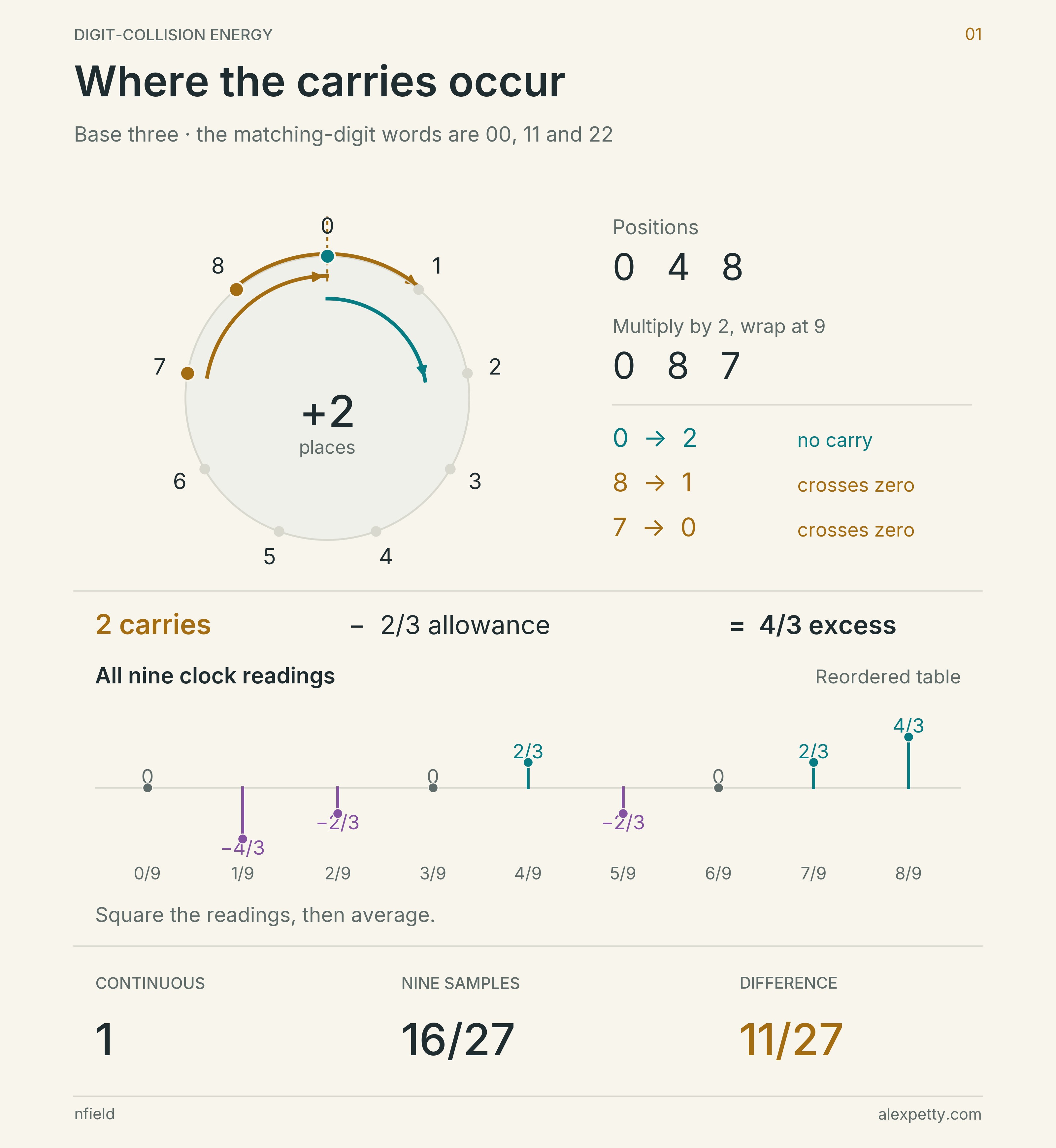
The picture’s lower half reads the same table a second way. Picture a quantity that climbs at a steady rate and falls back each time it reaches a whole number. Center it so it averages zero, and give it the value zero at the moment of the drop. That repeating ramp is a sawtooth, and I call it a clock. In base $p$ I run $p-1$ of them, the first going around once per unit, the second twice, the last $p-1$ times. Doubling each clock and adding them gives a single curve. Read that curve at the $p^2$ evenly spaced points of the grid and the readings are exactly the centered carry table, shuffled into a different order. The stems in the picture are the nine readings at base three, from $-4/3$ at the second point to $4/3$ at the last.

The energy now has two averages to compare. Square the nine stems and average them and you get $16/27$. Average the square of the whole curve and you get exactly $1$. The gold $11/27$ at the bottom is their difference, the sampling defect.

The two averages in the paper’s notation

Let $\psi(x)=\{x\}-1/2$ away from integers and $\psi(x)=0$ at integers. Here $\{x\}$ is the fractional part. Put $N=p-1$ and

$$B_N(x)=2\sum_{j=1}^{N}\psi(jx).$$

The continuous average and the grid average are

$$\mathcal J(N)=\int_0^1 B_N(x)^2 dx, \qquad \frac{E_p}{p^2}=\frac1{p^2}\sum_{a=0}^{p^2-1}B_N(a/p^2)^2.$$

Their difference is $\mathcal S_p=\mathcal J(p-1)-E_p/p^2$. The theorem proves $\mathcal S_p\to1$ through odd primes.

At base five the continuous average is $23/9$, the grid average is $48/25$, and the defect is exactly $143/225$.

Four clocks, one reset

Base five has four clocks and a grid of twenty-five points. In the upper half of the next picture each row is one doubled clock. The first rises once across the window and the fourth rises four times. Every one of them resets at zero, the shaded band on the left, because each goes around a whole number of times per unit.

Just to the right of zero each doubled clock sits near minus one, the open circle at the foot of its first ramp. Just to the left, coming around from the far end, each sits near plus one. The four add to nearly minus four on one side and nearly plus four on the other, so their square is close to sixteen on both sides. That is the open circle at the top of the peak in the lower graph. At zero itself each clock takes its assigned value zero, the gold dots in the shaded band, and the squared sum is zero. The grid samples exactly there. Its reading is the gold dot where the dashed line meets the axis, sixteen units below the curve on either side.

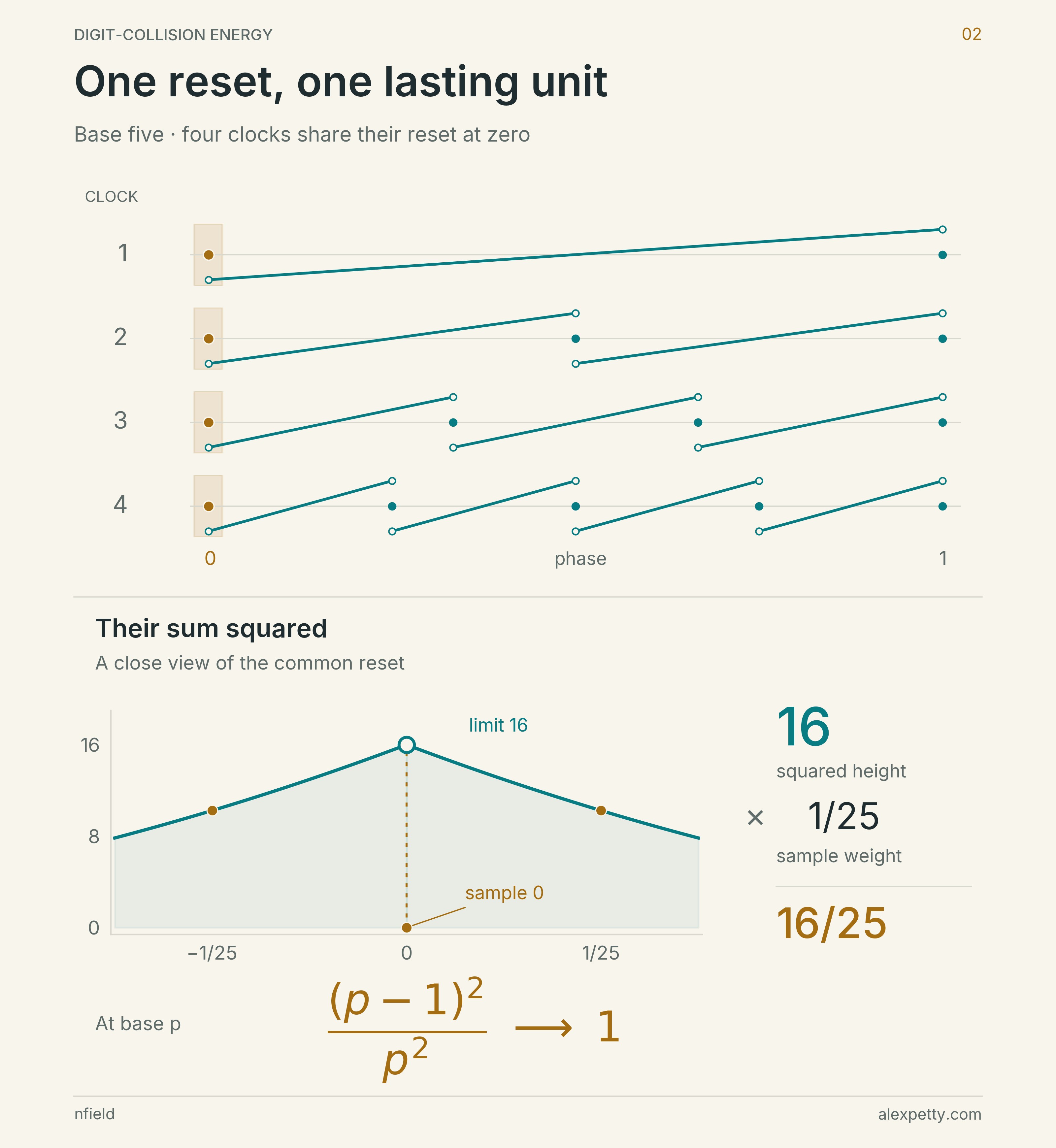
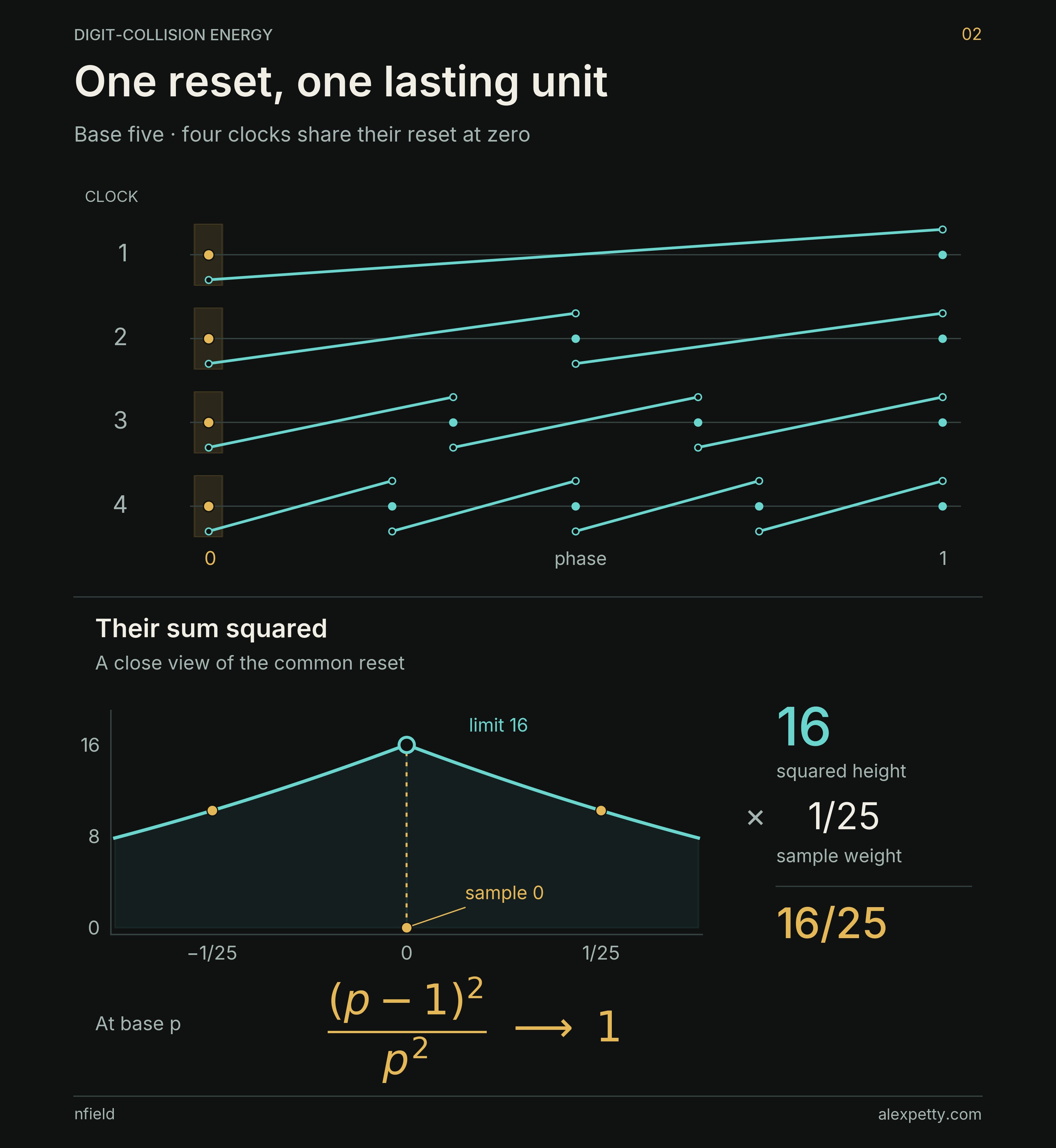
The curve’s average is the same whatever value sits at zero, since an integral cannot see one point. The grid gives that point a twenty-fifth of its average, and putting sixteen there in place of zero would raise the average by $16/25$, the number at the right. At base $p$ the peak is $(p-1)^2$ and the sample’s share is $1/p^2$, so the missing amount is

$$\frac{(p-1)^2}{p^2}\longrightarrow1.$$

The clocks are added before they are squared, and that is why this point never fades. Near zero they all agree, so the height of the peak grows with the square of the number of clocks, while the grid’s weight on one point shrinks as $1/p^2$. The two run at the same pace. With a fixed set of clocks and an ever finer grid, the missing sample would count for less and less, like any single point under an integral.

Twenty-five rectangles

Zero is the only place where every clock starts over together, but it is far from the only reset. A clock restarts wherever its frequency carries it to a whole number, and at each such point some clocks restart while the others carry on. At base five these are the smaller peaks and breaks at $1/4$, $1/3$, $1/2$, $2/3$ and $3/4$. Each one bends the curve in a way the grid may or may not catch, depending on where the reset falls between two sample points.

To see what they amount to together, put sixteen in place of the zero at the origin and leave every other sample alone. Draw each sample as a rectangle $1/25$ wide, standing on its own point and reaching to the right. The rectangles’ total area is the corrected grid average, and comparing them with the curve cell by cell shows every part of the difference that remains.

On the falling stretch at the left, each rectangle takes its height from the high end of its cell and overshoots the curve. Those cells are violet. On the rising stretch at the right, each rectangle takes the low end and falls short, and those cells are teal. The squared curve is symmetric about one half, so the tall violet bars opening the lower chart nearly mirror the tall teal bars that close it. The short bars between them belong to the interior resets.

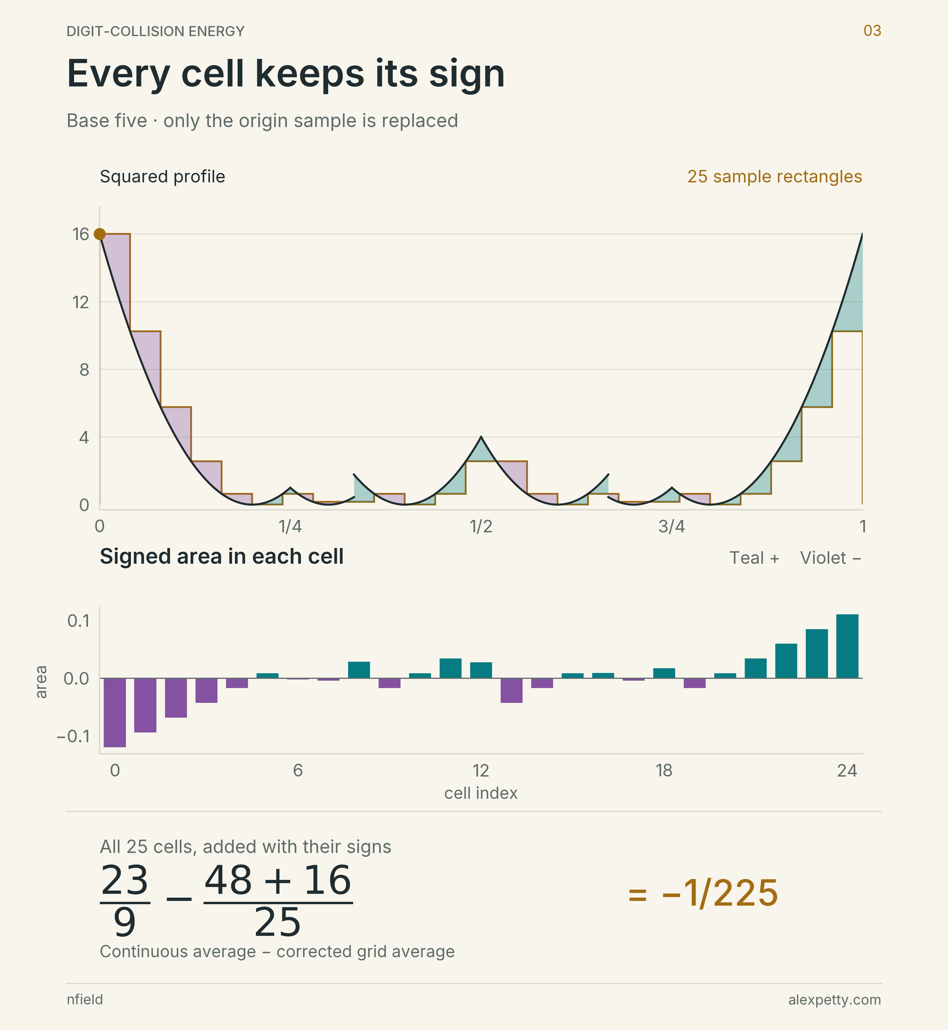
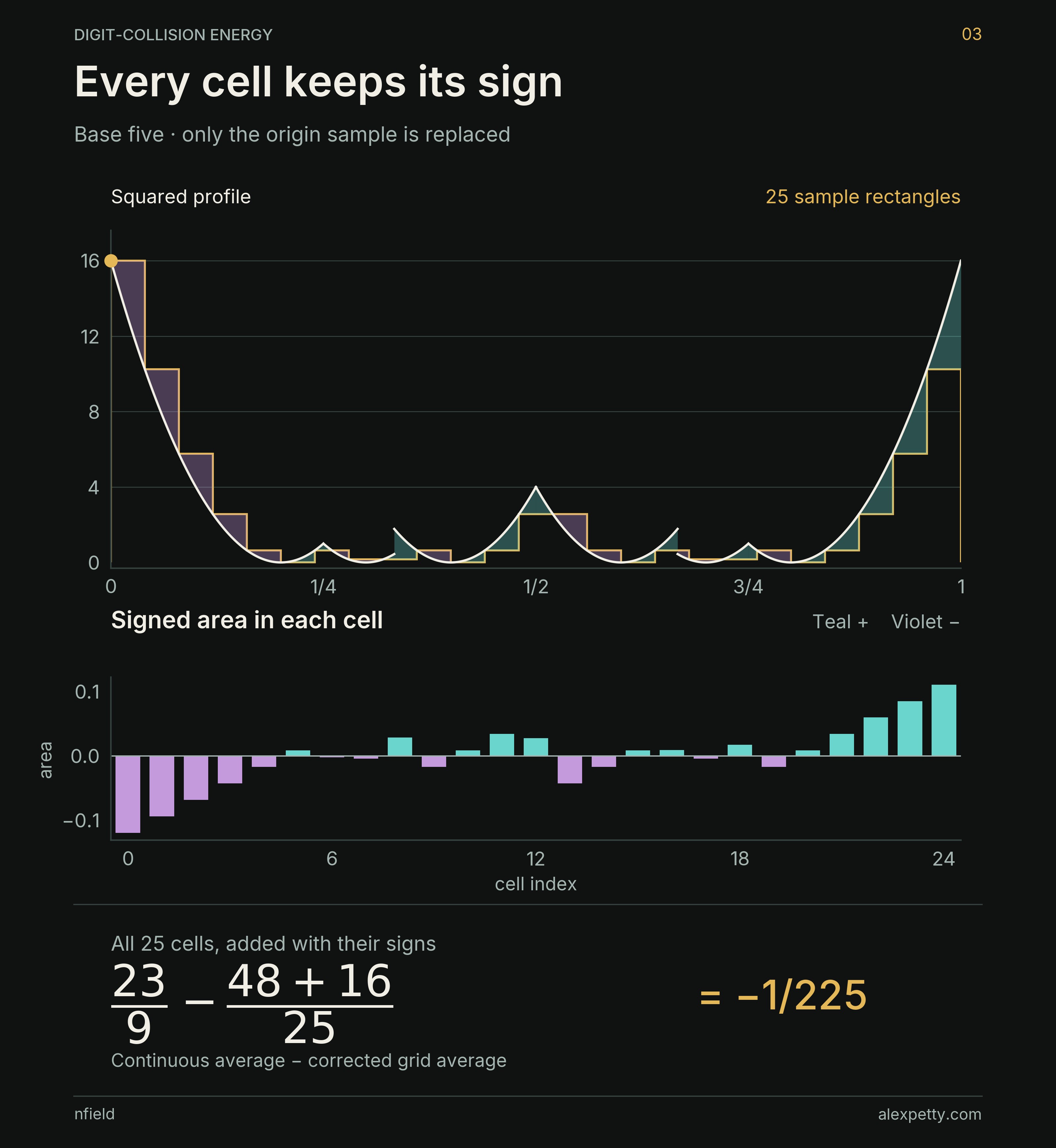
Add all twenty-five areas with their signs and the result is

$$\frac{23}{9}-\frac{48+16}{25}=-\frac1{225}.$$

Once the origin is corrected, the rectangles hold slightly more than the curve does. At other bases the leftover can fall on either side of zero, and the theorem proves that it tends to zero.

Two orientations in one wedge

Proving that the leftover vanishes is the hard part, and the proof spends nearly all its length there. The combined contribution of the interior resets can be written exactly as a signed sum of Dedekind sums, small finite sums that Richard Dedekind introduced in 1892, in his commentary on two of Riemann’s fragments about modular functions. They obey a reciprocity law. The Dedekind sum for a pair $(h, k)$ plus the one for $(k, h)$ equals a simple fraction.

Each use of that law is a division with remainder, much like a step of Euclid’s algorithm, and it trades one sum for an explicit correction and a new sum with a smaller modulus. Following every term down this way produces a large family of division paths. They have different lengths, and each comes in one of two orientations with opposite signs. Bounding the paths one at a time, by size alone, would throw away the cancellation between the orientations, and the proof needs that cancellation.

Each path can be rebuilt by a two-by-two matrix, and the top row of that matrix gives two whole numbers, $A$ and $B$. Their ratio always lands strictly inside one interval,

$$-\frac1{\varphi^2}<\frac BA<\frac1\varphi, \qquad \varphi=\frac{1+\sqrt5}{2},$$

from about $-0.382$ to $0.618$. In the other direction, every reduced fraction $B/A$ inside that interval, with $|B|$ at least two, comes from exactly one path. The endpoints come from the extreme division steps repeated forever, which turn $B/A$ into ratios of Fibonacci numbers closing in on the golden limits.

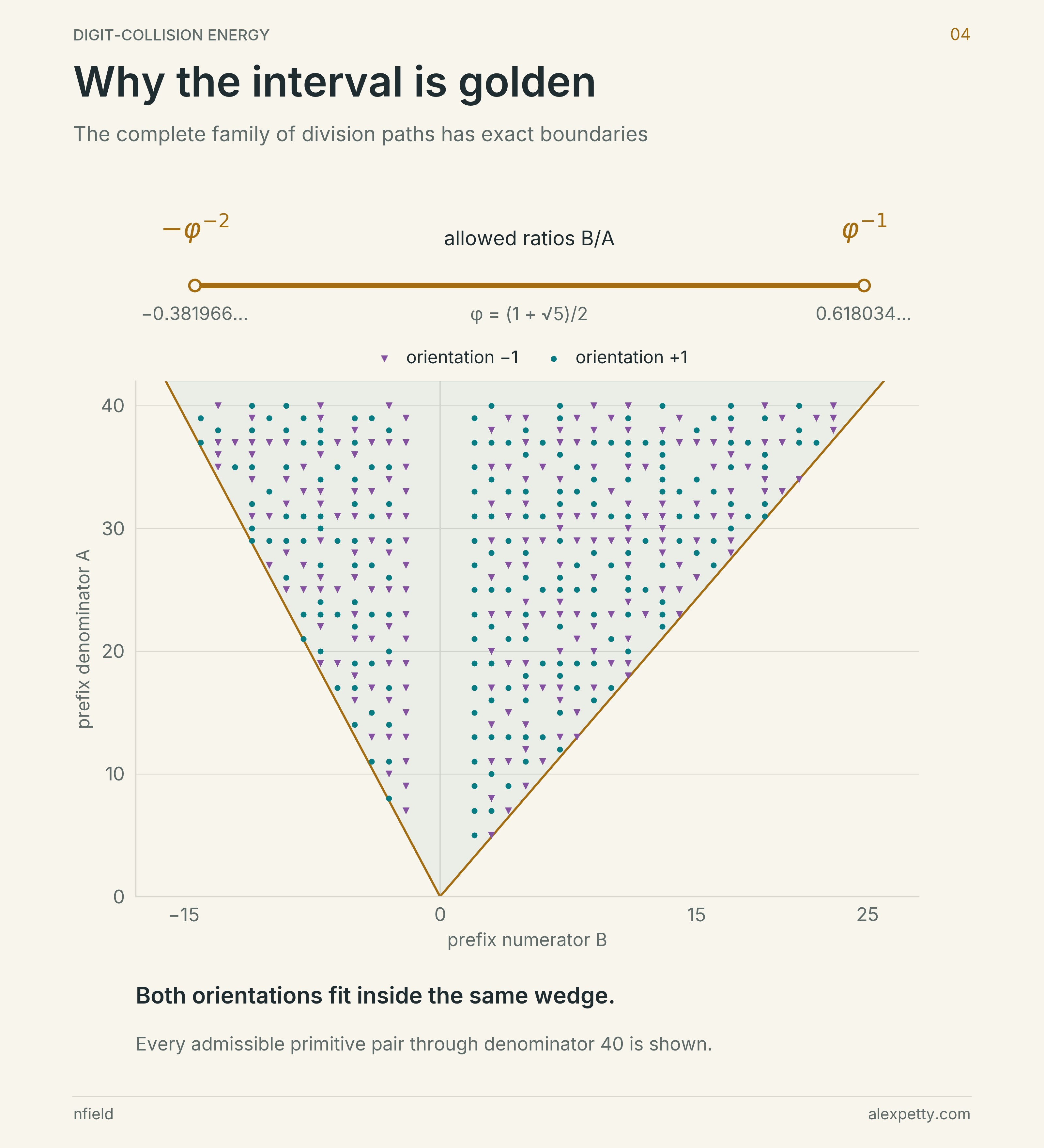
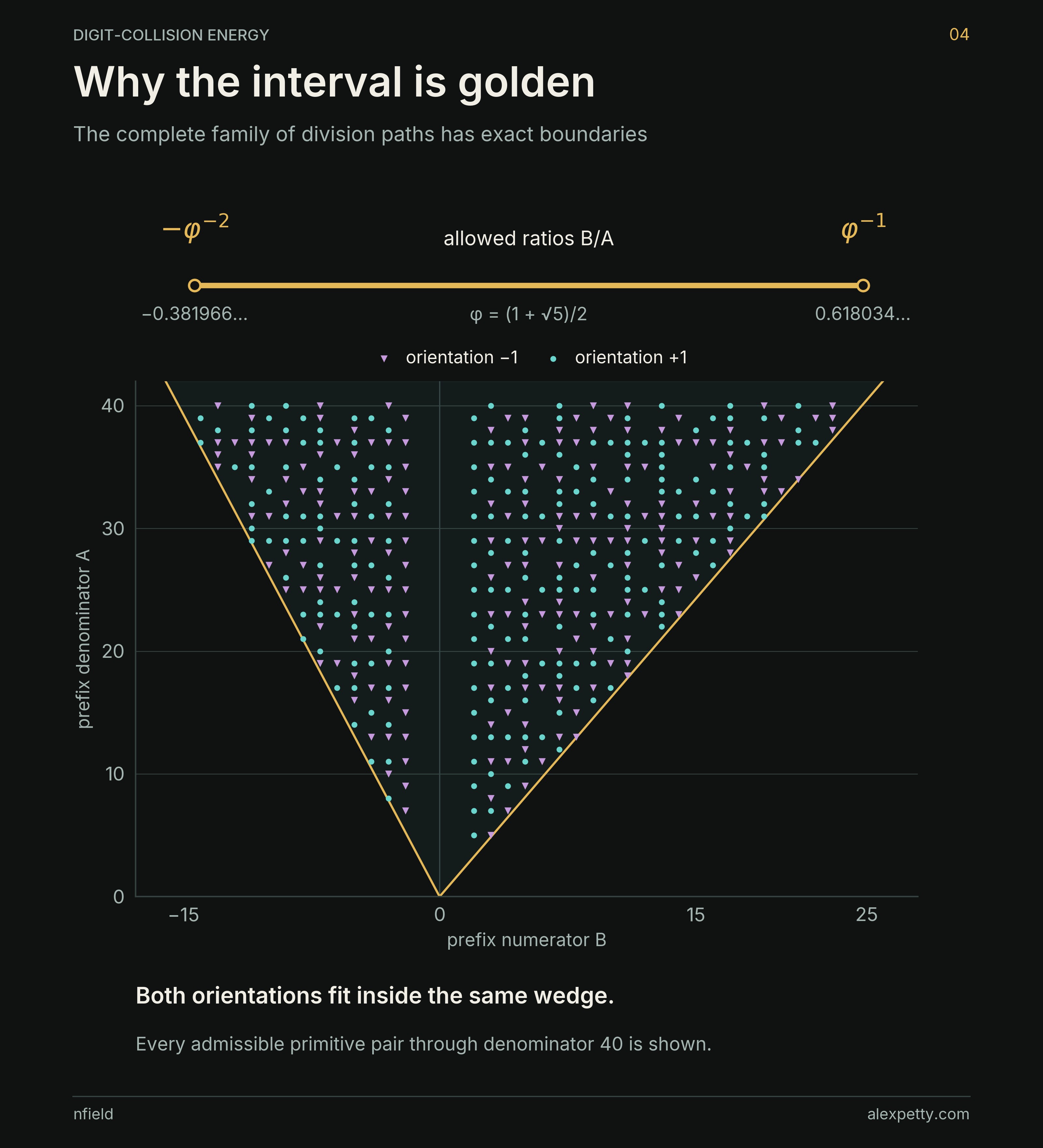
Each point in the picture is one path, with $B$ across and $A$ up. The two gold edges are the golden limits, and the lowest points sit at $A = 5$, the smallest denominator for a path of two or more steps. Circles and triangles are the two orientations. They are mixed together everywhere in the wedge, and neither claims a region of its own. An exact identity moves each path’s orientation sign into the reading it carries, so the two kinds can be summed as one population.

Once they are, hold $B$ fixed and walk up a single column of the wedge. Along that column the readings swing like a phase that depends on the reciprocal of $A$ plus a small shift, and classical estimates for sums of that kind show that they cancel by a small power of the base. The saving survives the sum over every starting cutoff and every depth of descent, which is what the limit requires.

The interval itself is classical. It is the shape of a family of continued fractions introduced by Hitoshi Nakada, and the paper proves directly the finite list of paths it needs. The golden ratio decides which paths exist. It has no part in the size of the unit, which comes from the reset at zero alone.

The rate the proof gives

The proved estimate is

$$\mathcal S_p=1+O\left(p^{-\eta}\log^4(2p)\right), \qquad \eta>0,$$

with an absolute implied constant. The exponent comes from two choices in the proof. Derivative estimates through order fourteen give a saving of $1/(2^{14}-2)$, and splitting the denominators at $p^{1/28}$ converts it to

$$\eta=\frac1{28(2^{14}-2)}=\frac1{458696}.$$

The exponent is a conservative choice, enough to make the error tend to zero. The golden interval is $((\sqrt5-3)/2,(\sqrt5-1)/2)$, and the unit itself comes from the separate ratio $(p-1)^2/p^2$.

Closing in on one

The last picture sets the theorem beside the tables. In the top panel the teal points are the full defect for every odd prime through 1,009 and for seven larger bases up to 10,007. They start at $0.41$ for base three, climb, and then scatter above and below the dashed line marking one, from about $0.87$ at base 73 to about $1.12$ at base 373. The gray curve beneath them is the reset alone, $(p-1)^2/p^2$, rising toward one. The lower panel takes that curve away. The violet points that remain are everything the interior resets do. They straddle zero, still swinging by a tenth among the bases below 1,000 and lying close to the line at the larger checkpoints.

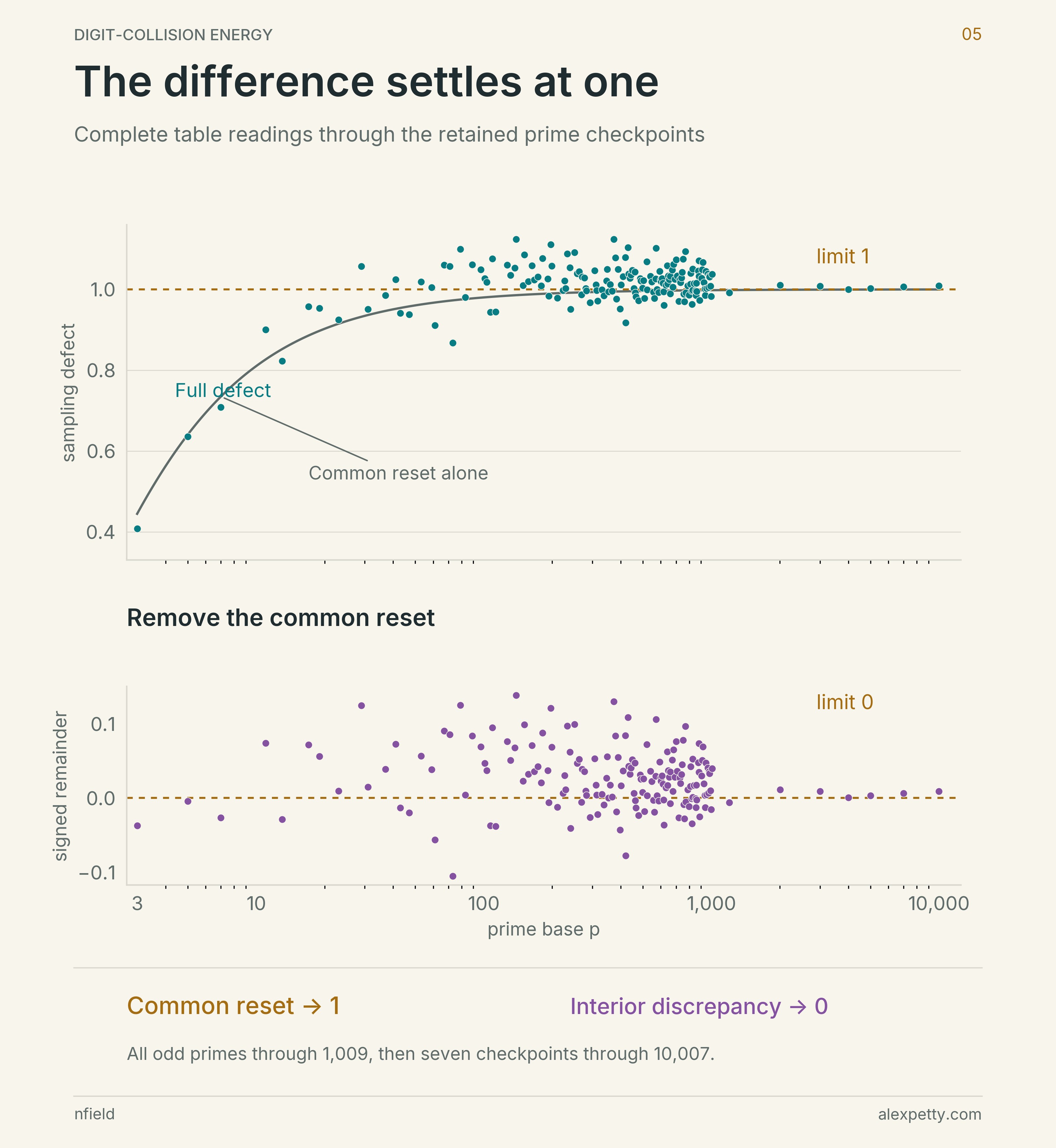
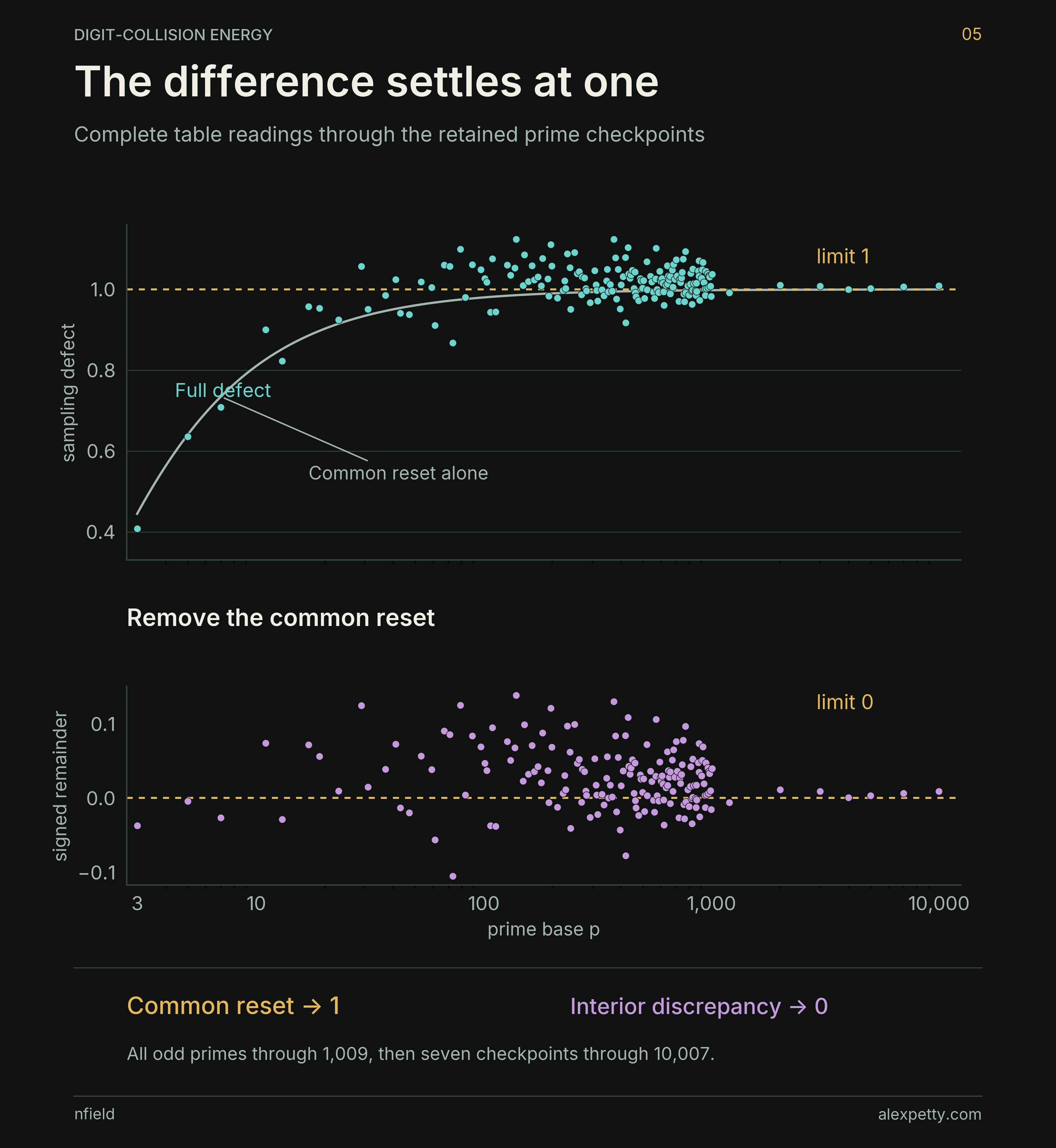
In energy units the theorem says

$$E_p=p^2\bigl[\mathcal J(p-1)-1\bigr]+o(p^2).$$

Digit Collisions and the Cubic Law gives the energy’s leading size, $p^3$, and The Secondary Term of the Cubic Law gives the next correction, of size $p^2(\log p)^2/\pi^2$. The unit found here sits beneath both, a correction of size $p^2$ measured against the exact continuous curve. It does not by itself give a third term of the energy’s expansion, which would also need a finer expansion of the curve’s own average.

The complete proof is in The Unit Sampling Defect in Digit-Collision Energy (PDF, preprint).

The proof’s rate is very slow. Its exponent, $1/458696$, is enough to force the limit and says almost nothing about speed. The tables suggest something much faster, a square-root rate,

$$\left|\mathcal S_p-1\right| =O_\varepsilon\left(p^{-1/2+\varepsilon}\right) \qquad\text{for every }\varepsilon>0.$$

The conjecture lets the defect wander above and below one. If it holds, the envelope around that wandering narrows about tenfold for every hundredfold increase in the base, apart from the small allowance $\varepsilon$. Proving it would take stronger cancellation within the same signed family of interior resets.

A million samples at base 1,009

Back at base 1,009, the grid has 1,018,081 samples and the curve has 308,925 interior resets inside the unit interval. The defect there is $1.03746$. The single sample at zero accounts for $0.99802$ of it, and all the interior resets together account for the remaining $0.03944$. As the base grows the second number tends to zero and the first tends to one. In the limit, the whole difference between the table and its curve comes from the one sample taken where every clock starts over.