Contents · four parts · 21 sections

Collision Calculus
Boundary Readings, Energy and Refinement

Alexander S. Petty

© 2026 Alexander S. Petty

Boston Agile Labs Press

October 2026

DOI: 10.5281/zenodo.23383403

Author’s Preface

I wanted a text I could return to after a year away and use to learn the calculations again. I also wanted readers interested in digit collisions, carry boundaries and arithmetic refinement to be able to follow the mathematics without reconstructing the earlier investigations. This book brings classical methods together with the constructions and estimates developed in that work.

The investigations began with finite arithmetic objects. Comparing their energies led to recurring questions about the relation between a finite table of readings and a continuous description of the same field. As the objects grew, their boundaries, coefficients and observation weights changed together. Unity supplied a fixed reference through those changes: a whole whose mass could be resolved into smaller shares, and a constant target whose unresolved part could be measured.

The difficulty often appeared at a small step in a larger calculation. A value assigned at a reset could change a sampled energy while leaving an integral unchanged. Components with separately understood energies could still have a substantial interaction. Moving a cutoff removed part of the old field, and that removed energy belonged in the same calculation as the new contribution. Each situation called for an exact account before an estimate could be trusted.

I have given this work the structure of a textbook so the techniques can be learned together. Worked examples make each convention explicit in a small calculation. Problems develop the reader’s command of the operations; the glossary and index keep the definitions accessible.

I use collision calculus for this coordinated method of boundary and energy calculation. The classical foundations and specific contributions are identified in Section 1.8.

The aim is practical. A reader should be able to take a new field, say how it is observed, choose an operation and determine what remains to be estimated. A line and three samples begin the text. Pulses and moving weighted signals then provide complete problems on which to learn the method. The arithmetic applications return to the questions that led me to gather these techniques in the first place.

Reader’s guide

Begin with the line and three readings in Section 1. Calculate their energies before following the general notation. Later operations extend that task to changing boundaries, components and weights. Section 1.3 introduces unity, conserved mass and the error in representing a fixed target.

Preparation. Parts I and II assume calculus, finite sums and elementary linear algebra. Begin with the real-valued examples; complex conjugates extend the operations to fields with phases. A finite positive measure can initially be read as a list of nonnegative sample weights. Theorem 4.1 uses Fourier series in its proof. A reader learning them can first work with its stated hypotheses, formula and examples, then return to the proof.

First reading. Read Sections 1–6 in order for the boundary data and mixed terms. Sections 7–11 show how to choose between boundary formulas, weighted primitives and invariant readings. The moving-window calculation in Section 10 and overlapping pulses in Section 11.2 combine these choices in complete examples. Follow how each specifies the observation, retains interactions and bounds any omitted tail.

Exercises and problems. Worked exercises demonstrate a method beside its solution. Pause at the question and try the first step before reading on. The separately numbered problems provide independent practice. Their hints and solutions are collected at the back (page 104); each answer links to its problem.

Reference use. The symbol table in Section 3 gives the notation; the glossary explains terms through definitions and examples. The index leads to their substantive uses. For a particular calculation, Section 2 handles changes of field and observation, Section 4 handles periodic boundaries, and Section 9 handles native weights and infinite tails. Section 11 collects the conditions needed when the field grows with the sampling scale.

Finite arithmetic. Part 3 develops collision registers, boundary budgets and transforms using congruences and finite sums. Divisor identities are derived where they enter. Prime counting illustrates the transform and the estimates required for recovery.

Growing-scale applications. Part 4 follows two fields through a change of scale. Carry grids lead to the half-cell limit, whose proof uses additional cited analytic estimates. Divisor families illustrate screening, whole-field refinement and invariant readings in three successive sections. Section 1.8 identifies the classical foundations and the specific constructions.

Part I. Boundary readings and sampled energy

1. Continuous and sampled energy

Suppose a periodic signal is known as a curve, but its energy is measured from a finite set of readings. An integral and a sample average are two ways of observing that signal. They need not give the same answer. This matters when a sampled energy is used to compare signals, choose a grid, or predict the effect of adding a new component. Before estimating their difference, we need to know which data each observation uses.

Here energy means squared magnitude, integrated or averaged. For a real reading $u$ it is $u^2$; for a complex reading it is $|u|^2$. Squaring makes interaction unavoidable. Two contributions of size one give an energy of four when they reinforce and zero when they cancel. Their separate energies add to two in either case.

The first calculation needs only a straight line, three sample points and the sum of their squares. It will identify three questions that recur throughout the subject. Which value is recorded at a boundary? Which components meet there? What changes when the observation is refined?

1.1. Reset values and sampled energy

On $0<x<1$, take the line $f(x)=2x-1$ and repeat it with period one. The value approaches $1$ before each integer and $-1$ after it. Assign the midpoint reading $f(0)=0$, and the same reading at every integer. These assigned values are part of the field.

Sample at $0,1/3,2/3$. The curve and the three readings are shown below. Open circles mark the limiting values at the ends of the rising segment; filled circles mark actual samples.

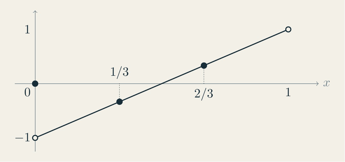
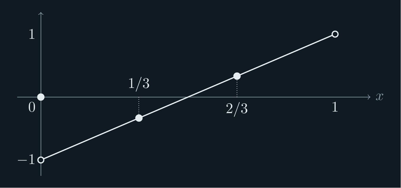
The continuous energy and the sampled energy are $$\int_0^1(2x-1)^2\,dx=\frac13,\qquad \frac13\left(0^2+\left(-\frac13\right)^2+ \left(\frac13\right)^2\right)=\frac2{27}.$$ Their difference, integral minus sample average, is $7/27$.

Now change only the reset reading to $g(0)=-1$. This is the right-hand reading of the same rising segments. Changing one point leaves the integral equal to $1/3$, but it increases the sample average by $1/3$. The two observations are

The same open curve has produced discrepancies of opposite signs. The integral and sample average are both correct for their definitions. The reading convention determines which comparison is being made.

1.2. Point contribution and signed remainder

At the reset, the two limiting energies are both one. Their average is one, whereas the midpoint reading has energy zero. A sampled point of weight $1/3$ therefore contributes $1/3$ to the discrepancy. The whole discrepancy is $7/27$, leaving a signed contribution of $-2/27$ from the rest of the boundary formula.

The point contribution has been separated from the complete answer. For the right-hand reading, the point contribution vanishes and the same $-2/27$ remains. Later, the derivative jump will account for that term.

1.3. Unity and refinement

Unity is the constant field $\mathbf 1(x)=1$. It gives a fixed reference while a description becomes more detailed. Both observations in the opening example assign total mass one: the interval has length one, and the three sample weights add to one. Consequently both assign energy one to unity. Their disagreement about the sawtooth comes from its readings at those same addresses.

A whole can be resolved into unequal shares. The reciprocal weights of the later native arithmetic observation are $$w_n=\frac1{n(n+1)}=\frac1n-\frac1{n+1},\qquad \sum_{n=1}^M w_n=1-\frac1{M+1}.$$ The last term tends to zero, so all positive addresses together have mass one. Resolving the first two addresses leaves $$1=\underbrace{\frac12}_{n=1} +\underbrace{\frac16}_{n=2} +\underbrace{\frac13}_{n\ge3}.$$ Resolving the next address divides the last share into $1/12+1/4$. The remaining $1/4$ still includes infinitely many addresses. It is part of the same total at every stage.

This is conservation of mass under subdivision.

If a cell of mass $m$ is partitioned into children of masses $m_1,\ldots,m_k$, then $$\sum_{j=1}^k m_j=m,\qquad \sum_{j=1}^k m_j|c|^2=m|c|^2.$$ The second identity follows when each child inherits the same reading $c$. Finer resolution alone has preserved that field’s energy. New child readings require a new energy calculation. The observation mass, the constant field unity and the energy of a general field are distinct objects. On an observation of mass one, the constant field two has energy four.

A resolved part and its complement.

Let $u_M(n)$ be one on addresses $1,\ldots,M$ and zero on all later addresses. This indicator field represents unity exactly on the resolved part. Its residual $r_M=\mathbf 1-u_M$ is one on the remaining tail. Their supports are disjoint, so $$\sum_{n\ge1}w_n|u_M(n)|^2=1-\frac1{M+1},\qquad \sum_{n\ge1}w_n|r_M(n)|^2=\frac1{M+1}.$$ For $M=2$, the represented energy is $2/3$ and the error energy is $1/3$. Admitting the third indicator transfers $1/12$ from the error to the represented part. The target remains $\mathbf 1$ throughout. Here the allowed fields are indicators; a prescribed clock family offers different corrections.

This fixed-target account motivates the refinement work in Unity, Refinement, and Signed Capture [6]. Section 9.1 develops its elementary clock example. Corrections there can overlap the old fit, so their signed interaction enters the error change. The mass partition identifies the whole being observed; the permitted fields determine how much of unity can be represented.

1.4. Collision amplitudes and interaction

Suppose a field has limiting values $u+v$ and $u-v$ on the two sides of a boundary, with the midpoint value $u$ recorded at the boundary. The average of the limiting squared magnitudes is $|u|^2+|v|^2$. The recorded square is $|u|^2$. Their local difference is $|v|^2$.

If several components reset together, their signed jumps add before this square is taken. This coincidence of boundary events is a collision. Its contribution depends on the combined reading, including the interaction between the resetting components.

For example, add a second copy of the three-sample field $f$. The combined field is $2f$, whose discrepancy is $4(7/27)=28/27$. Adding the two individual discrepancies gives only $14/27$. The missing $14/27$ is the mixed contribution. If the second field is $-f$ instead, the combined field and its discrepancy vanish. The mixed contribution then cancels the two individual discrepancies.

Both calculations are consequences of $$|f+g|^2=|f|^2+2\operatorname{Re}(f\overline g)+|g|^2.$$ The mixed term must be observed using the same integral or sampling rule as the two squares, including when that rule changes.

1.5. Grid refinement and field growth

For the same midpoint field $f$, now sample at $a/q$, $0\le a<q$. Elementary sums of integers and their squares give $$\frac1q\sum_{a=1}^{q-1}(2a/q-1)^2 =\frac13-\frac1q+\frac{2}{3q^2}.$$ The discrepancy is therefore $$D_q[f]=\frac1q-\frac{2}{3q^2}\longrightarrow0.$$(1) Here $D_q$ is simply a name for integral minus sampled mean square. The field was held fixed while the grid changed.

Now let the field grow with that grid: $f_q=\sqrt q\,f$. Both observed energies are multiplied by $q$, so the complete discrepancy is $$D_q[f_q]=1-\frac{2}{3q}\longrightarrow1.$$(2) This limit has been calculated directly, including its signed remainder. There is no conflict with the fixed-field limit. The changing amplitude has exactly offset the decreasing weight of one sample.

A collision of $m$ equal components has squared amplitude proportional to $m^2$. On a $q$-point grid its point contribution can consequently have size $m^2/q$. This explains why the scale $m\asymp\sqrt q$ deserves attention. In a general growing family the remaining signed terms still require an estimate; formula (2) works because those terms were also computed.

1.6. Interval pulse

Take a unit pulse supported on $[1/4,3/4)$ and sample at $0,1/4,1/2,3/4$. The continuous energy is the interval length $1/2$. Two of the four readings are one, so the sampled energy is also $1/2$. The discrepancy is zero.

Change the pulse to have value zero at both endpoints. The integral stays $1/2$, but only the sample at $1/2$ remains. The sampled energy is now $1/4$ and the discrepancy is $1/4$. This calculation uses the same point-replacement rule as the clock example. Rising segments and arithmetic divisibility are not required for that operation.

The later pulse calculation allows any interval, amplitude, endpoint readings and grid offset. It will show how a boundary formula replaces a fresh case-by-case count each time the sampling grid moves.

1.7. Changes of field and observation

The starting question is concrete: how does an observed squared norm change when its field or observation changes? The data needed for an answer depend on that change.

These operations matter whenever an integral is used to compare or predict a finite squared observation. The examples will cover periodic signals, interval indicators, arithmetic carry fields and reciprocal address weights. Each application specifies its observation before applying the common rules.

1.8. Classical foundations and specific contributions

The general operations come from established analysis and linear algebra. Their classical names identify the mathematics being used.

The point-value rule is the contribution of an atom to an integral. The positive midpoint term is the parallelogram identity. The localization rule compares two nonnegative tail energies. Each is derived here in the form needed for the calculations; its elementary basis remains visible.

Unity in Section 1.3 is the usual constant function one. Its approximation uses weighted squared error, and its mass partitions use additivity of the observation. The arithmetic setting and the distinction between resolving a reading and admitting a new clock come from the refinement work [6].

The contribution of the general presentation is to put these operations on the same specified field and observation. A boundary reading, a combined reset, a moved sampling grid and a changed activation cutoff can then be followed through one calculation. The clock formula makes that organization explicit through the collision amplitude, inherited reading and slope. The moving-window and pulse examples show how to turn the identities into complete answers for growing families.

Sections 12–15 collect tools developed in the square-root sampling investigation. The signed register, finite-column estimate and interior norm construction retain that investigation’s specific arithmetic data. Primitive-shell grouping and the logarithmic transform express classical divisor operations in a reusable form; their application to the clock remainder supplies the finite prime-counting identity. The derivations are included here.

The specialized results have a more particular provenance. The unshifted carry limit comes from The Unit Sampling Defect in Digit-Collision Energy [5]. The half-cell source reduction, parity transfer and quarter-limit are developed in Section 17, using analytic estimates from that work. They are the principal new arithmetic development of this manuscript.

The native screening constant $129$, cycle-alignment credit and parent-shell constructions were developed in the divisor-field investigation. Sections 18–20 derive them from the prescribed family profiles and include their proofs. The quadratic cutoff is an explicit application of the general localization rule. The four-reading construction specializes constrained energy to the later divisor families. Its failed sufficiency comparison at the four stated cutoffs is an exact result of the present investigation. These are specific formulas, constructions and estimates, with their derivations and dependencies identified. Collision calculus names this coordinated method of boundary and energy accounting.

For the next problem, a grid with $q$ points and offset $\theta$ samples $(a+\theta)/q$, $0\le a<q$. The offset is measured in cells: $\theta=1/2$ moves each sample by half a cell, or $1/(2q)$.

2. Fields and observations

A field supplies readings. An observation assigns mass to the addresses at which those readings are taken. Here an address is simply a location in the domain, such as a point of an interval or an integer index. Keeping both objects visible lets the same calculation describe a grid, an interval integral, a moving window or an infinite weighted tail.

A two-address example separates the two objects. Give the readings $1,3$ masses $1/2,1/2$. The observed energy is $(1^2+3^2)/2=5$. Keep the readings but change the masses to $3/4,1/4$; the energy becomes $3$. Keep those new masses and change the second reading to $1$; the energy becomes $1$. The first change belongs to the observation, the second to the field. We need notation that records both.

For a finite table, the definitions below reduce to these weighted sums. A measure records the mass assigned to each measurable set of addresses. Its integral adds readings with those masses, extending the same operation to a continuous profile or an infinite weighted tail.

Let $X$ be a measurable address space whose singletons are measurable. An observation $\rho$ is a finite positive measure on $X$; its mass need not be one. A field is a specified measurable function on $X$, including its readings at atoms of $\rho$. Define $$Q_\rho h=\int_X h\,d\rho,\qquad E_\rho[f]=Q_\rho(|f|^2), \qquad K_\rho(f,g)=Q_\rho(f\overline g).$$ We use $Q_\rho$ only when the integral exists and use $E_\rho$ and $K_\rho$ on fields of finite energy. Cauchy–Schwarz then gives $|K_\rho(f,g)|^2\le E_\rho[f]E_\rho[g]$. The ordinary letters describe the operation; subscripts describe the observation. These are the usual integral, squared norm and mixed form for the chosen measure. Their value here is that the observation stays explicit when its addresses or masses change.

When two observations $\rho,\sigma$ are compared, write $$D_{\rho,\sigma}[f]=E_\rho[f]-E_\sigma[f],\qquad K_{\rho,\sigma}(f,g)=K_\rho(f,g)-K_\sigma(f,g).$$ Both fields must have finite energy in both observations. The difference $D$ can have either sign. It is quadratic in the field, and its mixed form $K_{\rho,\sigma}$ need not be positive.

Here $\delta_x$ assigns mass one to the single address $x$. Thus an entry $v\delta_x$ in the observation means “read at $x$ with weight $v$.” A collection of such point masses turns the integral into the corresponding weighted sum.

In the grid setting the first comparison measure is understood to be $dx$, so $D_{q,\theta}$ and $K_{q,\theta}$ abbreviate these two-measure operations. Later $E_S$ abbreviates the native tail. Normalizing a tail to mass one would define a different observation and change its energy.

2.1. Energy under changes of field and observation

Suppose the old experiment observes $f$ with $\rho$, and the new one observes $f+g$ with $\sigma$. The field $f$ must be specified at every new address, even where the old observation assigned no mass.

The three terms answer different parts of the calculation. The first charges the old field for changing its observation. The second measures the new field’s signed interaction with what was already present. The third is the new field’s own energy.

For a small calculation, give addresses $1,2,3$ old masses $(1/2,1/3,1/6)$ and new masses $(0,1/2,1/2)$. Take $f=(1,2,0)$ and $g=(0,-1,1)$. The energies are $11/6$ and $1$. The three terms on the right are respectively $1/6,-2,1$. Their sum is $-5/6$. Removing address one does not determine the answer by itself; reweighting address two and its negative mixed term also contribute.

2.2. Readings, superposition and consistency

If two fields differ only on an at most countable set $A$, have finite energy, and agree elsewhere, then $$E_\rho[g]-E_\rho[f] =\sum_{a\in A}\rho(\{a\})\bigl(|g(a)|^2-|f(a)|^2\bigr).$$ This is the general point-value replacement rule. Its series is absolutely convergent. An atomless observation ignores the changed readings; an atomic observation charges their actual masses.

For finitely many components $f=\sum_jc_jf_j$, the matrix $G_{ij}=K_\rho(f_j,f_i)$ gives $E_\rho[f]=c^*Gc$. Here a collision means that components contribute at a common observed address; the mixed term measures their interaction. Components with disjoint observed support have zero mixed energy. Components meeting at a boundary contribute through their combined reading. The interaction may reinforce or cancel in the combined energy.

Changing an experiment in two stages gives a useful consistency check. Apply (3) to each stage and add. The intermediate energy cancels, leaving the direct change. The allocation among the three terms can depend on the chosen intermediate field and observation; their total cannot. This check catches a lost shell or a duplicated boundary credit before any estimate is attempted.

3. Fields, traces and sampled energy

The first example distinguished a curve from its assigned readings. We now record that distinction for any periodic field with finitely many boundaries. Work on $\mathbb T=\mathbb R/\mathbb Z$, the unit interval with its ends identified. Write $\lfloor x\rfloor$ for the greatest integer at most $x$, $\lceil x\rceil$ for the least integer at least $x$, and $\{x\}=x-\lfloor x\rfloor$ for the fractional part. The notation $\mathbf 1_A$ is one on the set $A$ and zero elsewhere.

An admissible field $f:\mathbb T\to\mathbb C$ has a finite set $\mathcal B$ of specified boundary points. On each open arc between consecutive points of $\mathcal B$, it extends to a $C^2$ function on the closed arc. The extensions from adjacent arcs may differ. The actual value $f(b)$ is specified separately at every $b\in\mathcal B$. Include isolated exceptional readings in $\mathcal B$, even if the two traces agree. A smooth field may be given an artificial boundary at zero.

The $C^2$ condition means that the function and its first two derivatives are continuous on each closed piece. It permits integration by parts inside each piece while keeping its endpoint terms. A trace is the limiting value reached from one side. In the opening sawtooth, the left trace at zero is $1$, the right trace is $-1$, and the assigned reading is $0$. These are three distinct pieces of data.

For any function $h$ with these properties, write $$[h]_b=h(b+)-h(b-),\qquad \langle h\rangle_b=\frac{h(b+)+h(b-)}2,\qquad a_b(h)=\langle h\rangle_b-h(b).$$ All traces at zero are periodic traces. The notation $h''_{\rm reg}$ means the ordinary second derivative on the open arcs, ignoring the finitely many boundary points. The point data are not identified modulo sets of measure zero.

For an integer $q\ge1$ and $0\le\theta<1$, define $$X_{q,\theta}=\left\{\frac{a+\theta}{q}:0\le a<q\right\},\qquad Q_{q,\theta}h=\frac1q\sum_{a=0}^{q-1}h\left(\frac{a+\theta}{q}\right).$$ The linear sampling discrepancy and the quadratic energy defect are $$L_{q,\theta}(h)=\int_0^1h\,dx-Q_{q,\theta}h, \qquad D_{q,\theta}[f]=L_{q,\theta}(|f|^2).$$ We abbreviate $Q_{q,0}$ and $D_{q,0}$ to $Q_q$ and $D_q$. The square is taken before sampling. Define the periodic kernels $$\psi(t)=\begin{cases}\{t\}-1/2,&t\notin\mathbb Z,\\0,&t\in\mathbb Z,\end{cases} \qquad \widetilde B_2(t)=\{t\}^2-\{t\}+\frac16.$$ The first kernel takes its midpoint value at a jump. The second is continuous. Their respective absolute bounds are $1/2$ and $1/6$. Ordinary letters $Q,D,K$ denote sampling, energy defect and mixed defect. The offset may be suppressed only after its value has been fixed. The kernels will record where a boundary falls within a sample cell. For a boundary $b$, the number $qb-\theta$ is an integer precisely when the boundary is sampled. Its fractional part records the relative position otherwise. Thus the apparently global sampling problem has local phase data at each boundary.

3.1. Boundary data

The periodic integral identifies functions that differ at finitely many points. A finite sampling rule need not do so. For example, let $f$ vanish everywhere except at zero, where $f(0)=a$. Then $$\int_0^1|f|^2\,dx=0,\qquad D_q[f]=-\frac{|a|^2}{q}.$$ Both traces at zero vanish. The entire defect comes from the specified point value. This field is admissible after zero is included in $\mathcal B$. If the grid misses zero, its defect is zero as well.

The two measures being compared are Lebesgue measure and the atomic measure $q^{-1}\sum_{x\in X_{q,\theta}}\delta_x$. Their difference is a signed measure. A positive defect means the continuous energy exceeds the sampled energy; a negative defect means the sampled energy exceeds the continuous energy. Neither sign is prescribed in advance.

3.2. Point-value replacement

This identity permits a calculation to use a convenient trace convention and then restore the required readings exactly. The correction depends on the grid: changing an unsampled point has no effect.

4. Boundary decomposition

The three-sample calculation had a point contribution and a signed remainder. The following formula separates that remainder into value jumps, slope jumps and curvature between boundaries. Its four terms can be calculated from local data before any asymptotic estimate is made.

Euler–Maclaurin summation supplies the underlying relation between sums, integrals and boundary data. Its circular formulation treats interior and periodic jumps [2]; shifted sampling with jumps is developed by Berrut and Trummer [3]. The Bernoulli kernels used below are defined in Section 3 and their Fourier expansions enter the proof. The purpose here is to teach how actual readings and quadratic interactions enter that relation, and how to preserve them through changes of observation.

For use of the formula, there are four entries to prepare. At each boundary record the actual energy and its two traces, then the two slope traces. Between boundaries retain the ordinary second derivative. The grid supplies the phase $qb-\theta$ at each boundary. The theorem weights those entries by two fixed periodic functions. Its first term records only boundaries actually sampled; the remaining terms account for the surrounding profile. The proof derives those weights from Fourier series, but the calculation itself uses the listed local data.

The proof uses a different description of the same data. Integration by parts records the jumps in each Fourier coefficient. Averaging a Fourier mode over the grid removes it unless its frequency is a multiple of $q$. Summing the surviving modes produces the two Bernoulli kernels. The point replacement at the end restores the actual boundary readings. This is why the formula needs both the surrounding traces and the specified values.

The midpoint of a field and the midpoint of its energy are different readings. At an integer-zero sawtooth reset the field takes its midpoint, so its energy is smaller than the midpoint of the two energy traces. The resulting point correction is positive. The signed terms in (4) need not be positive.

This is an absolute sufficient condition. A growing arithmetic family may require cancellation in the signed sums when their absolute bounds do not decay. The decomposition identifies those sums without supplying an estimate for them.

4.1. Polynomial curvature

Let $f(x)=x^2$ on $0\le x<1$ and extend it periodically, retaining $f(0)=0$. Its energy profile is $h(x)=x^4$ on that interval. At the periodic join, the boundary data are $$a_0(h)=\frac12,\qquad [h]_0=-1,\qquad [h']_0=-4, \qquad h''_{\rm reg}(x)=12x^2.$$ On the unshifted $q$-grid the value-jump term vanishes because $\psi(0)=0$. The point and derivative terms are $1/(2q)$ and $-1/(3q^2)$. To calculate the regular term, split the integral into the $q$ cells and set $qx=a+t$ in cell $a$. Since $$\int_0^1\widetilde B_2(t)\,dt=\int_0^1t\widetilde B_2(t)\,dt=0, \qquad \int_0^1t^2\widetilde B_2(t)\,dt=\frac1{180},$$ direct expansion gives $$\int_0^1 x^2\widetilde B_2(qx)\,dx =\frac1{q^3}\sum_{a=0}^{q-1}\int_0^1(a+t)^2\widetilde B_2(t)\,dt =\frac1{180q^2}.$$ Thus the complete answer is $$D_q[f]=\frac1{2q}-\frac1{3q^2}+\frac1{30q^4}.$$ For $q=2$ it is $27/160$. Directly, the squared integral is $1/5$ and the two sampled squares have mean $1/32$, giving the same result. The $q^{-4}$ contribution would disappear if regular curvature were discarded. This example follows the full procedure from the specified reading to the boundary data, the regular integral and a direct check.

5. Simultaneous arithmetic resets

For clocks, the local data have a particularly simple form. Each reset has a known jump, and each open segment has a constant slope. Simultaneous resets must first be grouped into a single signed amplitude. The clock $2\psi(2x)$ repeats the opening ramp twice during one trip around the circle, resetting at zero and one half. In a general clock $2c\psi(rx+\phi)$, $r$ counts repetitions, $\phi$ chooses the phase, and $c$ sets the signed or complex amplitude. The three parameters change different parts of the boundary calculation.

Let $r_1,\ldots,r_s$ be positive integers, let $\phi_1,\ldots,\phi_s\in\mathbb T$, and let $c_1,\ldots,c_s\in\mathbb C$. Set $$F(x)=2\sum_{j=1}^s c_j\psi(r_jx+\phi_j),\qquad V=2\sum_{j=1}^s c_jr_j.$$ Let $\mathcal B$ be the union of all reset locations. At $b\in\mathcal B$ define the collision set and its amplitude by $$I_b=\{j:r_jb+\phi_j\in\mathbb Z\},\qquad C_b=\sum_{j\in I_b}c_j.$$ The nonreset reading is $U_b=2\sum_{j\notin I_b}c_j\psi(r_jb+\phi_j)$. Every location is counted once, with all its resetting clocks included in $I_b$.

For unit coefficients, a collision of $m$ clocks contributes $m^2/q$ if the grid samples it. With general coefficients, $$|C_b|^2=\sum_{j\in I_b}|c_j|^2 +2\operatorname{Re}\sum_{\substack{j<k\\j,k\in I_b}}c_j\overline{c_k}.$$ The reset budget already contains interference. Two clocks with the same frequency and phase and coefficients $1,-1$ have zero total field and zero collision amplitude at every reset. A count of individual resets alone would miss this cancellation.

5.1. Two resetting clocks

For $F=2\psi(x)+2\psi(2x)$, the slope on every open segment is $V=6$. The distinct boundary locations are zero and $1/2$. Their data are $$\begin{array}{c|ccc} b&C_b&U_b&V\\ \hline 0&2&0&6\\ 1/2&1&0&6 \end{array}$$ Thus the interaction term vanishes at both locations. On the unshifted nine-point grid, only zero is sampled, and $$\sum_b C_b\widetilde B_2(9b)=2\widetilde B_2(0)+\widetilde B_2(1/2)=\frac14.$$ The clock formula gives $$D_9[F]=\frac49-\frac{12}{81}\frac14=\frac{11}{27}.$$ On the half-cell grid, only $1/2$ is sampled. Now $$\sum_b C_b\widetilde B_2(9b-1/2) =2\widetilde B_2(1/2)+\widetilde B_2(0)=0,$$ and $D_{9,1/2}[F]=1/9$. The continuous field has not changed. The two sampling rules select different collision amplitudes.

Phase shift and inherited interaction.

The zero interaction above comes from its particular reset locations. Shift the second clock and take $$F(x)=2\psi(x)+2\psi(2x+1/4).$$ The slope is still $V=6$, but the nonreset readings now contribute. The complete boundary data are $$\begin{array}{c|rrrr} b&C_b&U_b&F(b-)&F(b+)\\ \hline 0&1&-1/2&1/2&-3/2\\ 3/8&1&-1/4&3/4&-5/4\\ 7/8&1&3/4&7/4&-1/4 \end{array}$$ At every reset the actual reading is $F(b)=U_b$. On the unshifted two-point grid, only zero is a sampled reset. Also $\psi(3/4)=1/4$ and $\widetilde B_2(3/4)=-1/48$, so the three terms of (7) are $$\underbrace{\frac12}_{\text{sampled reset}} +\underbrace{2\left(-\frac14\frac14+\frac34\frac14\right)}_{ \text{inherited interaction}} -\underbrace{3\left(\frac16-\frac1{48}-\frac1{48}\right)}_{ \text{slope contribution}} =\frac12+\frac14-\frac38=\frac38.$$ The actual samples are $F(0)=F(1/2)=-1/2$, giving sampled energy $1/4$. For an independent integral check, the three open segments are $$F(x)= \begin{cases} 6x-3/2,&0<x<3/8,\\ 6x-7/2,&3/8<x<7/8,\\ 6x-11/2,&7/8<x<1. \end{cases}$$ Integrating their squares gives $27/128+13/32+1/128=5/8$. Thus the defect is $5/8-1/4=3/8$, as the boundary formula gives. Dropping the inherited term would give $1/8$. Its contribution comes from the two unsampled boundaries, through the nonreset readings there.

5.2. Clock boundary calculation

For a clock family with specified coefficients, list distinct reset locations before taking any squares. At each location, sum the coefficients of the resetting clocks to obtain $C_b$, and evaluate only the nonreset clocks to obtain $U_b$. The global slope $V$ is computed once. A boundary is sampled exactly when $qb-\theta$ is an integer. These data supply all three terms of (7).

This procedure also provides a useful diagnostic. If the amplitudes of two resetting clocks cancel, their joint point correction disappears, but their interactions at other boundaries must still be evaluated. Cancellation at one location does not remove either clock from the field.

5.3. Reset-reading exercise

6. Interval pulses and endpoint conventions

A pulse asks a counting question. How many of the sample addresses fall inside its interval, and are the endpoints admitted? Moving an endpoint changes the integral continuously, but a sampled reading changes when the endpoint passes it. The boundary formula describes both effects using the same two endpoint locations.

The same theorem applies to a field with two boundaries and no rising clock segments. Fix $0<\alpha<\beta<1$ and $A\in\mathbb C$. Let $f=A$ on $(\alpha,\beta)$ and $f=0$ outside $[\alpha,\beta]$. Specify $f(\alpha)=u$ and $f(\beta)=v$ independently.

For a fixed amplitude and fixed endpoint readings, the defect is $O(q^{-1})$ uniformly in the grid offset. A persistent defect can be produced by growing the amplitude. Let $q$ tend to infinity through multiples of three, take $\alpha=1/3$, $\beta=2/3$, $\theta=0$ and $A_q=\sqrt{\lambda q}$ with $\lambda\ge0$. Both endpoints lie on the grid. The four conventions below have identical continuous energy.

These values follow directly from (8). They show why a constant defect belongs to a specified family and reading convention. No universal nonzero constant is forced by discreteness alone.

Overlapping pulses also retain their interactions. For half-open intervals $I_j$, let $f=\sum_j A_j\mathbf 1_{I_j}$. Then the energy contains $2\operatorname{Re}(A_j\overline{A_k})\mathbf 1_{I_j\cap I_k}$ for each pair $j<k$. Formula (11) keeps these overlap contributions. Their boundaries may coincide even when the intervals themselves differ.

6.1. Overlap exercise

Part II. Field and observation changes

7. Boundary calculations

The choice of operation depends on the data available. Write the observed energies, then choose the formula whose required data can be evaluated or bounded.

7.1. Readings and changed data

Give the addresses, their masses and the actual readings. A native tail beginning after $S$ starts at $S+1$. Write a changed field as $f+g$ on the union of old and new addresses. The following choices determine which additional data the calculation needs.

An energy change may first be decomposed and its mixed term then bounded by summation by parts. The weighted calculation follows.

7.2. Observation weights and primitive sums

Cancellation can be visible in a running total even when the individual terms are large. For $u(1),\ldots,u(4)=(1,-1,1,-1)$, the running totals are $1,0,1,0$. Against arbitrary readings $x_1,\ldots,x_4$, $$\sum_{n=1}^4u(n)x_n=(x_1-x_2)+(x_3-x_4).$$ Constant partners cancel completely. Slowly changing partners leave only their changes. Summation by parts extends this calculation to any sequence, with its final running total supplying an endpoint term.

On a uniform periodic grid, the Bernoulli kernels in Theorem 4.1 move the calculation onto point readings, jumps and regular derivatives. For an arbitrary weighted sequence, ordinary summation by parts is the corresponding operation. If $T(n)=\sum_{k=a}^n u(k)$, $T(a-1)=0$, and $x_n$ is any complex sequence, then finite telescoping gives $$\sum_{n=a}^b u(n)x_n =T(b)x_b+\sum_{n=a}^{b-1}T(n)(x_n-x_{n+1}).$$(10) Indeed, substitute $u(n)=T(n)-T(n-1)$ and shift the second finite sum; its lower endpoint vanishes because $T(a-1)=0$. For mixed energy take $x_n=v_n\overline{g(n)}$, where $v_n$ is the observation mass. Its difference is $$x_n-x_{n+1} =(v_n-v_{n+1})\overline{g(n)} -v_{n+1}\overline{g(n+1)-g(n)}.$$ Both the mass variation and the field variation remain.

With an unanchored primitive $F$, the lower endpoint is $-F(a-1)x_a$. Subtracting $F(a-1)$ from the primitive redistributes that endpoint across the formula. It cannot remove a contribution to the observed energy. At an infinite upper endpoint, write the finite identity first and prove that its endpoint tends to zero.

7.3. Uniform estimates and signed work

If $|T(n)|\le P$, (10) gives $$\left|\sum_{n=a}^b u(n)x_n\right| \le P\left(|x_b|+\sum_{n=a}^{b-1}|x_n-x_{n+1}|\right).$$ The primitive bound measures cancellation in $u$; the bracket measures the variation of its weighted partner. For a growing family, write both as functions of its scale. A small primitive for each component is useful only after the number, amplitudes and interactions of those components have also been counted.

If this absolute estimate is too large, return to the signed identity. Its parent-shell term can be negative. Its mixed work can cancel a new square. Taking absolute values before those terms have been joined changes the estimate being sought.

8. Interaction, refinement and dilation

The opening calculation showed that adding two fields also adds their interaction. We now make that interaction an operation, then track what happens when the sampling grid changes.

For admissible fields $f,g$ on a common boundary partition, define $$K_{q,\theta}(f,g) =\int_0^1f\overline g\,dx-Q_{q,\theta}(f\overline g).$$ For real fields this is simply the discrepancy of their pointwise product. For complex fields the conjugate gives $K(g,f)=\overline{K(f,g)}$, with the grid subscripts understood. The form is linear in its first input; scaling its second input by $c$ scales the result by $\overline c$. These properties are called Hermitian symmetry and sesquilinearity. The mixed form need not be positive. Linearity gives $$D_{q,\theta}[f+g] =D_{q,\theta}[f]+D_{q,\theta}[g] +2\operatorname{Re}K_{q,\theta}(f,g).$$(11) Theorem 4.1 applies directly to $f\overline g$, so it also resolves each mixed contribution into boundary and regular terms.

8.1. Collision matrix

With many components, repeating a two-field expansion becomes cumbersome. A matrix stores the result of every pairwise comparison. Its diagonal records individual defects, and its off-diagonal entries record the mixed defects. Choosing the component amplitudes then selects one quadratic expression from this table. For two identical real fields of defect $d$, all four entries are $d$; amplitudes $(1,1)$ give $4d$, while $(1,-1)$ give zero.

Let $f_1,\ldots,f_s$ be admissible. For $z\in\mathbb C^s$, put $F_z=\sum_{j=1}^s z_j f_j$ and define $$G^{\rm cont}_{jk}=\int_0^1\overline{f_j}f_k\,dx, \qquad G^{\rm grid}_{jk}=Q_{q,\theta}(\overline{f_j}f_k), \qquad H=G^{\rm cont}-G^{\rm grid}.$$ Both Gram matrices are positive semidefinite. Their difference can have either sign.

The matrix formulation separates two useful facts. Collision point corrections are nonnegative for midpoint readings. The full defect also contains the signed matrix $H-P$. A basis change reorganizes both matrices. It does not by itself estimate $H-P$, or require equal energy in different coordinates. Character transforms can be used as unitary coordinate changes when their normalization and underlying finite space are specified; additional symmetry is needed for any stronger conclusion.

8.2. Grid refinement and dilation

The six-point grid separates into two three-point grids. Its even indices give $0,1/3,2/3$, and its odd indices give $1/6,1/2,5/6$. The six-point average is therefore the mean of the two three-point averages. This is the first identity below.

Dilation changes the arguments read by the grid. Sampling $f(2x)$ at those same six addresses reads $f$ at $0,1/3,2/3$, each twice. Only three distinct readings remain. In general the greatest common divisor of the dilation and grid size counts these repetitions.

For a fixed field, averaging over all grid offsets also gives $$\int_0^1D_{q,\theta}[f]\,d\theta=0.$$ Indeed the substitution $x=(a+\theta)/q$ turns the offset average of $Q_{q,\theta}|f|^2$ into its continuous integral. A persistent defect along a specified aligned grid is compatible with this identity.

As a direct check on the role of resonance, take $F(x)=2c\psi(mx+\phi)$. Put $\alpha=\{m'\theta+q'\phi\}$ as above. For the unit-frequency field $2c\psi$, the only boundary has $U_0=0$, $C_0=c$ and $V=2c$. Thus $$D_{q,\theta}[F] =|c|^2\left(\frac d q\mathbf 1_{\{\alpha=0\}} -\frac{4d^2}{q^2}\widetilde B_2(\alpha)\right).$$(14) For $q=m$ and zero phases this is $|c|^2/3$, since every sample is a reset. For fixed $m,c,\phi$ it tends to zero as $q\to\infty$.

For a unit clock with $c=1$, the unshifted and half-cell formulas are particularly simple: $$D_q[2\psi]=\frac1q-\frac{2}{3q^2},\qquad D_{q,1/2}[2\psi]=\frac1{3q^2}.$$ At offset $\theta=1/8$, the same field instead has defect $-11/(48q^2)$. These expressions all tend to zero, while having different signs and different leading orders. The jump at an exactly aligned offset is the contribution of its specified reset reading.

8.3. Joint field and grid refinement

Equation (12) holds with the field fixed. Suppose the new field is $f+g$ and the new grid has $rq$ points. Combining refinement with polarization gives $$\begin{aligned} D_{rq,\theta}[f+g] ={}&\frac1r\sum_{j=0}^{r-1}D_{q,(j+\theta)/r}[f] +D_{rq,\theta}[g]\\ &+2\operatorname{Re}K_{rq,\theta}(f,g). \end{aligned}$$ The new field contributes its own defect and its interaction with the old field. This is the appropriate identity when refinement adds clocks or changes amplitudes. A grid identity alone would omit those terms.

8.4. Algebraic rules

Fix the grid and write $D$ and $K$ with its subscripts suppressed. For scalars $c,d$ and admissible fields, $$\begin{aligned} D(cf)&=|c|^2D(f),\\ K(cf,dg)&=c\overline d\,K(f,g),\\ D(f+g)&=D(f)+D(g)+2\operatorname{Re}K(f,g). \end{aligned}$$ These follow by expanding the squared magnitude or mixed product before either observation. Point changes use Proposition 3.1. Grid refinement and dilation use Proposition 8.2; translation is its case $m=1$, with new offset $\{\theta+q\phi\}$. Write $$P_{q,\theta}(f)=A_{q,\theta}(|f|^2),\qquad R_{q,\theta}(f)=D_{q,\theta}[f]-P_{q,\theta}(f).$$ Then $D=P+R$ separates the sampled point contribution from the remaining signed work. Each rule keeps the same field, grid and reading conventions unless their change is explicitly included.

8.5. Coordinate and resonance exercises

8.6. Invariant readings

An addition can change every sample while leaving one combination of samples fixed. That fixed reading can force energy to remain. Take three equally weighted addresses and the field $f=(0,1,0)$. Permit any affine addition $h(i)=a+bi$. The second difference $$L(f)=f(1)-2f(2)+f(3)$$ annihilates every such addition, so $L(f+h)=-2$. Cauchy–Schwarz gives $$|L(f+h)|^2\le(1^2+(-2)^2+1^2)\sum_{i=1}^3|f(i)+h(i)|^2.$$ Consequently the observed energy is at least $2/3$. The constant addition $h=-1/3$ attains that value, leaving $(-1/3,2/3,-1/3)$. The permitted additions can remove the affine part of the readings; the remaining bend has a definite energy cost.

Here the weights are one, so energy is a sum rather than a normalized mean. Changing the weights changes the cost of preserving the same reading. With weights $(1,2,1)$, the lower bound becomes one and is attained by the addition $h=-1/2$.

This is weighted Cauchy–Schwarz used as a refinement rule. First specify the permitted additions, then construct a reading that all of them annihilate. Its value is inherited from the old field. The denominator records how much energy is required to carry that value under the actual observation weights. No sign condition is imposed on the individual field components.

8.7. Joint invariant readings

Several invariant readings may use the same addresses. Their interaction must then be retained, just as it is for the original fields. The task is to find the least energy compatible with all the retained readings at once. Let the rows of a matrix $A$ be their coefficients, so $Af$ is the list of retained values, and let $W=\operatorname{diag}(w_i)$ record the cost of each address. The condition $\ker A=V$ says that these readings detect every change outside the allowed space. When some such changes remain undetected, the same formula still gives a lower bound, but need not be attained by an allowed addition.

This is the classical minimum-norm problem under linear constraints , written in the coordinates of the invariant readings. The joint matrix measures their overlap in the reciprocal weights. Adding their separate lower bounds without this matrix can count the same retained energy twice.

9. Native weights and moving fields

An equally weighted periodic grid and an activated arithmetic tail observe a field in different ways. Summation by parts remains the classical tool. The task here is to carry the actual observation, reset reading and field change through it. Here native means that the weights are prescribed by the arithmetic observation.

The first three native masses are $1/2,1/6,1/12$. The later readings continue indefinitely, with decreasing mass. A constant unit field has energy one over all positive addresses, but energy $1/2$ after the first address is removed. That change occurs before the field itself has changed. The weights are $$w_n=\frac1{n(n+1)}=\frac1n-\frac1{n+1},\qquad \sum_{n\ge a}w_n=\frac1a.$$ For an integer $S\ge0$, define the native energy and mixed observation $$E_S[p]=\sum_{n>S}w_n|p(n)|^2,\qquad \langle p,v\rangle_S=\sum_{n>S}w_np(n)\overline{v(n)}.$$ The cutoff is part of the observation. It excludes $S$ and begins at $S+1$. A finite clock field is bounded, so its energy is finite for every fixed cutoff. No uniform bound in a changing clock family follows from this assertion alone.

The weights also have an exact geometric reading. For the step interpolation $\widehat p(u)=p(\lfloor u\rfloor)$, $$E_S[p]=\int_{S+1}^{\infty}\frac{|\widehat p(u)|^2}{u^2}\,du =\int_0^{1/(S+1)} |p(\lfloor1/x\rfloor)|^2\,dx.$$(18) Each address cell has mass $\int_n^{n+1}u^{-2}\,du=w_n$. Thus the infinite tail consists of reciprocal cells accumulating at zero. Formula (18) is an identity of observations, not a limiting approximation by equally weighted samples.

The cell $(1/(n+1),1/n]$ has length $w_n$. At $S=2$, the retained cells $n\ge3$ fill the interval $0<x\le1/3$. The entire infinite tail is present in this finite interval; its cells become progressively shorter near zero. Individual endpoints have no effect on the integral in (18).

9.1. Approximation of unity

The reciprocal cells make the unity account of Section 1.3 geometric: they partition $(0,1]$, and $\mathbf 1(n)=1$ is the constant reading on every cell. Thus $E_0[\mathbf 1]=1$, whereas $E_S[\mathbf 1]=1/(S+1)$. Activation retains the mass of the selected tail. Renormalizing that tail would change the observation.

For $N\ge2$, let a clock approximation and its residual be $$p_N(n)=\sum_{j=2}^N c_{N,j}\{n/j\},\qquad r_N(n)=\mathbf 1(n)-p_N(n),\qquad \mathcal R_N=E_0[r_N].$$ The coefficients may change as more clocks become available, while unity remains the same target. Every such finite field is bounded, so its complete error is finite. At a common multiple of its periods, all fractional clocks read zero. The residual there reads one and has positive native mass. Thus every finite clock approximation leaves positive error.

For an added finite clock field $h$, the new residual is $r_N-h$. Expanding its square gives the complete error change $$E_0[r_N-h]-E_0[r_N] =E_0[h]-2\operatorname{Re}\langle r_N,h\rangle_0.$$ All terms converge by boundedness and summability of the weights. An improvement requires the residual’s signed response to pay for the correction’s energy. Several corrections must be combined before their cost is squared. If the old and new coefficients minimize error over nested clock spaces, the minimum cannot increase, because the old fit is still available. A prescribed coefficient change must instead be assessed by the displayed identity.

The first fractional clock.

The clock $\phi_2(n)=\{n/2\}$ reads $1/2$ on odd addresses and zero on even addresses, including every reset. The odd addresses have mass $\log2$. To see the infinite sum directly, for $M\ge1$ write $$\sum_{k=1}^M w_{2k-1} =\int_0^1\frac{1-x^{2M}}{1+x}\,dx \longrightarrow\int_0^1\frac{dx}{1+x}=\log2.$$ The omitted integral is nonnegative and at most $1/(2M+1)$. The even addresses therefore have mass $1-\log2$. For a real coefficient $c$, the complete squared error is $$E_0[\mathbf 1-c\phi_2] =\log2\,(1-c/2)^2+1-\log2.$$ It is minimized at $c=2$. The fit equals unity at every odd address; its residual equals unity at every even address. Their energies are $\log2$ and $1-\log2$. This is a partition of the original target over the complete observation, with actual right-hand clock readings at every reset [6].

These comparisons keep the observation $E_0$ fixed. A moving activation cutoff also removes old readings; Proposition 9.3 retains that additional contribution.

9.2. Reciprocal-weight boundary terms

For the constant reading one, the identity $w_n=1/n-1/(n+1)$ makes successive terms cancel. Between $a$ and $N$ only $1/a-1/(N+1)$ remains. A changing reading interrupts that cancellation by its successive differences. The next formula retains those interruptions and both endpoints.

Write $\Delta h(n)=h(n)-h(n-1)$ for a backward difference.

For energy, put $h=|p|^2$ and $a=S+1$. A bounded clock field therefore has a complete boundary account beginning with $|p(S+1)|^2/(S+1)$. The combined differences $\Delta|p|^2$ must be kept together in the ordered limit. Separating a positive jump-square series from its mixed series can produce two divergent sums even when their joined series converges.

For interaction estimates it is more useful to move the difference onto the weighted partner. Define the anchored primitive $T_a(n)=\sum_{k=a}^n u(k)$, with $T_a(a-1)=0$.

For a conjugate mixed observation, replace $v$ by $\overline v$. The first interior term is caused by variation of the weights. It is present even when the partner field is constant.

9.3. Right-hand clocks and combined resets

At integer addresses, the clock $\{u/3\}$ repeats the readings $0,1/3,2/3$. At three it resets to zero, while its left trace is one. A sum of such clocks is specified by a coefficient table, called its source. Here $q(j)$ is the coefficient of the clock of length $j$; it is a function of $j$, distinct from the grid size $q$ used earlier. At address $n$, precisely the lengths dividing $n$ reset together.

Let $q(j)$, $j\ge1$, be a finitely supported complex source. Define $$p(u)=\sum_jq(j)\{u/j\},\qquad \sigma=\sum_j\frac{q(j)}j,\qquad c(n)=\sum_{j\mid n}q(j).$$ At an integer address $n$, the actual reading is the right-hand value. The traces and discrete increment satisfy $$p(n)=p(n+),\qquad p(n-)=p(n)+c(n),\qquad \Delta p(n)=\sigma-c(n).$$(23) Indeed each fractional clock rises by $1/j$ between successive integer addresses and subtracts one exactly when $j\mid n$. If the source is reciprocally neutral, $\sigma=0$. The slope then vanishes on every open unit cell, $p(n-)=p(n-1)$, and the combined signed reset is $\gamma(n)=-c(n)$.

For a neutral source the complete energy jump is $$\Delta|p(n)|^2 =2\operatorname{Re}\bigl(\overline{p(n-1)}\gamma(n)\bigr) +|\gamma(n)|^2.$$(24) The divisor contributions are added in $c(n)$ before taking a square. Its square contains every interaction between simultaneous resets. The other term is their work against the inherited reading. Substituting their joined expression into (20) preserves the ordered boundary account.

The same rule for two complex fields is $$\begin{aligned} \Delta(X\overline Y)(n) ={}&X(n-1)\overline{\Delta Y(n)} +\overline{Y(n-1)}\Delta X(n)\\ &+\Delta X(n)\overline{\Delta Y(n)}. \end{aligned}$$ It retains both inherited readings and the simultaneous jump product. All these identities follow by expanding the new reading as the old reading plus its increment.

9.4. Point-value correction at resets

For two sequences with finite native energy, the point-value replacement rule is $$E_S[g]-E_S[f]=\sum_{n>S}w_n\bigl(|g(n)|^2-|f(n)|^2\bigr).$$(25) Only changed readings contribute. The series is absolutely convergent, since its absolute terms are bounded by the two energy series. This extends Proposition 3.1 to the weighted infinite set. The sign is the change in sampled energy; it is opposite to the change in an integral-minus-sample defect when the integral is fixed.

At a reset put $m_n=(p(n+)+p(n-))/2$ and $\gamma_n=p(n+)-p(n-)$. The actual right reading is $m_n+\gamma_n/2$, so $$\begin{aligned} |p(n+)|^2-|m_n|^2 &=\operatorname{Re}(m_n\overline{\gamma_n}) +\frac14|\gamma_n|^2,\\ a_n^+(|p|^2) :=\frac{|p(n-)|^2+|p(n+)|^2}{2}-|p(n+)|^2 &=-\operatorname{Re}(m_n\overline{\gamma_n}). \end{aligned}$$(26, 27) The midpoint correction $|\gamma_n|^2/4$ has been adjusted by the change in the squared reading. The resulting right-hand correction can have either sign. For a neutral finite clock field, both the midpoint and right-hand sequences are bounded, so (25) applies to all their reset addresses. The midpoint is formed from the same clock field, not by silently replacing its fractional clocks with centered clocks.

Activation has its own boundary. If $b_S(n)=\mathbf 1_{\{n>S\}}p(n)$, then for $n\ge1$ $$\Delta b_S(n)=\mathbf 1_{\{n=S+1\}}p(S+1) +\mathbf 1_{\{n\ge S+2\}}\Delta p(n).$$(28) The first admitted reading is not generally the raw clock’s reset at that address. The activation term records the whole admitted field.

9.5. Field increments and activation

There are two changes to follow. The moved cutoff removes old readings on $S<n\le T$. Beyond $T$, the old field is still present when the addition arrives. Subtracting the removed energy and expanding the retained square gives the complete change. In particular, a positive new square can be outweighed by the removed shell or a negative interaction.

The negative parent shell contains the square of the entire old field. If that field is a sum of families, their shell interactions are inside the same square. If the change is a sum, its square likewise contains all interactions between changed families. A shorter observation window or a separate bound for the new square does not replace (29).

9.6. Two-clock native tail

Consider $$p(u)=\{u\}-2\{u/2\}.$$ Its reciprocal source sum is $1-2/2=0$. At integer addresses, $p(n)=-1$ for odd $n$ and $p(n)=0$ for even $n$. The formal clock of length one has zero reading at every integer, but its source coefficient is needed for neutrality and for the reset formula.

At address one the left and right readings are $0,-1$. The midpoint reading is $-1/2$, with midpoint energy correction $1/4$. The actual right-hand correction is $1/2-1=-1/2$. At address two the readings are $-1,0$ and the right-hand correction is $1/2$. Thus positive midpoint corrections cannot be used unchanged even in this two-clock example.

The complete energy is $$E_0[p]=\sum_{r\ge0}\frac1{(2r+1)(2r+2)}=\log2.$$ To evaluate the tail exactly, write each summand as $\int_0^1x^{2r}(1-x)\,dx$. Nonnegativity permits summation under the integral, giving $\int_0^1(1+x)^{-1}\,dx=\log2$. Now double the field and move the cutoff from $S=0$ to $T=1$. The change is $v=p$. Formula (29) gives $$E_1[2p]-E_0[p] =-\frac12+2\left(\log2-\frac12\right) +\left(\log2-\frac12\right)=3\log2-2.$$ The three terms are the removed parent shell, the inherited interaction, and the new square. Directly, $E_1[2p]=4(\log2-1/2)$, which gives the same answer. Every later address is included in both calculations. Here every raw jump has squared magnitude one, so the separate boundary series $\sum_n|\gamma(n)|^2/n$ diverges. Its mixed counterpart cancels that divergence in the ordered energy-jump series. The joined boundary expression is the convergent object.

9.7. Weighted tail localization

The same two-clock example illustrates how a finite calculation can enclose a complete observation. Stop its changed energy at $N=4$. The removed parent reading contributes $-1/2$, and the only admitted odd address is three. The finite answer is $$H_4=-\frac12+\frac3{3\cdot4}=-\frac14.$$ Every omitted term lies between zero and $3w_n$. The remaining weight is $1/(N+1)$, giving $$-\frac14\le 3\log2-2\le-\frac14+\frac35=\frac7{20}.$$ Stopping at eight gives $H_8=-27/280$ and the interval $[-27/280,199/840]$. The finite answer may have the wrong sign while its enclosure remains valid. A tail allowance is part of the answer.

This calculation extends to an arbitrary positive observation on the integer addresses. The old and new fields can grow with an outside parameter; their envelopes determine how far the observation must run.

The square of the complete new field gives the upper allowance; the square of the complete old field gives the lower allowance. Expanding the omitted work and bounding its mixed terms separately would usually give a larger enclosure. In the two-clock calculation, the known sign and the identity $|2p|^2-|p|^2=3|p|^2$ improve both sides further.

For a family with envelopes $A_S,C_S$, an error at most $\epsilon$ is guaranteed by $$N\ge T,\qquad N+1\ge \frac{\max(A_S^2,C_S^2)}{\epsilon}.$$ An envelope proportional to $S$ therefore permits localization at a constant multiple of $S^2$. The cutoff grows with the field. No fixed-field quadrature constant is being used as a uniform estimate.

10. Growing signals in weighted windows

Consider a receiver whose observation window moves farther along a sequence while a rapidly alternating component becomes larger. Each sample has a specified mass. The question is whether the observed energy has a stable limit, and whether the oscillation’s interaction with the background survives.

The observation in this model has its own weights, specified below; they are not replacements for the native masses. Fix positive integers $a<b$, a bounded weight $\rho\ge0$, and real functions $A,B$ on $[a,b]$. At scale $N$ observe the addresses $aN<n\le bN$ with masses $$v_{N,n}=N^{-2}\rho(n/N).$$ The total mass is $O(N^{-1})$. Let $u(n)$ be a real carrier signal and set the actual readings $$f_N(n)=B(n/N)+\sqrt N\,A(n/N)u(n).$$ The carrier term has growing amplitude. Its square is multiplied by an observation whose mass shrinks at the compensating rate.

10.1. Four-sample window calculation

Take $a=1$, $b=2$, $\rho(x)=x^{-2}$ and $A=B=1$, with $u(n)=(-1)^n$. The masses are $v_{N,n}=1/n^2$. At $N=4$ the four addresses are $5,6,7,8$, their readings are $-1,3,-1,3$, and $$E_4=\frac1{25}+\frac9{36}+\frac1{49}+\frac9{64}.$$ The result is $35361/78400$. A continuous-address version holds each reading on $[n,n+1)$, so these are its actual right-hand readings. Write $U_N=\sum_{N<n\le2N}n^{-2}$ and $V_N=\sum_{N<n\le2N}(-1)^n n^{-2}$. Then exactly $$E_N=(N+1)U_N+2\sqrt N\,V_N.$$(32) The first part contains the background square and the carrier square. The second retains their signed interaction.

At $N=9$ the window becomes $10,\ldots,18$ and the readings alternate between $4$ and $-2$. To compare these observations, extend the formula $f_N(n)=1+\sqrt N(-1)^n$ to all positive addresses. The change field is $f_9-f_4=(-1)^n$. Formula (3) gives $$E_9-E_4 =-E_4+\sum_{n=10}^{18}\frac{f_4(n)^2}{n^2} +2\sum_{n=10}^{18}\frac{f_4(n)(-1)^n}{n^2} +\sum_{n=10}^{18}\frac1{n^2}.$$ The removed old window, admitted old readings, mixed term and new square all appear. The windows happen to be disjoint here; the general identity also handles overlap and changes of weight on retained addresses.

The estimate below is an application of classical summation by parts and bounded-variation quadrature. Its role is to expose every constant for this moving observation, so the growing amplitude can be handled without a fixed-field assumption.

10.2. Uniform bound for growing amplitude

The slowly varying envelopes also need a quantitative description. Total variation adds the magnitudes of successive changes along a partition and takes the supremum over all partitions. A monotone function has variation equal to its endpoint difference in magnitude; for example, $x^{-2}$ on $[1,2]$ has variation $3/4$. Oscillation and jumps both consume variation. This is the quantity that the primitive estimate charges to the partner of the rapidly alternating carrier.

For a specified function $h$ of bounded variation on $[a,b]$, put $$\|h\|_{\rm BV,*}=|h(b)|+\operatorname{Var}_{[a,b]}h.$$ Variation includes the assigned point readings. This convention allows step envelopes and exceptional endpoint values. Suppose the three products $$h_0=\rho B^2,\qquad h_1=\rho AB,\qquad h_2=\rho A^2$$ are of bounded variation. Their Lebesgue integrals are well defined. They correspond to the background square, the mixed product and the carrier square. The constants $P$ and $R$ below control the running sums of the carrier and of its squared fluctuation about $c$. For the alternating carrier, the first running sum stays small and the squared fluctuation vanishes identically. These two controls serve different terms in the energy expansion.

The alternating carrier has $P=1$, $c=1$, $R=0$. For the four-sample example all three products equal $x^{-2}$ on $[1,2]$. Their variation is $3/4$, their $\|\cdot\|_{\rm BV,*}$ is one, and their integral is $1/2$. Thus every positive integer $N$ satisfies $$\left|E_N-\frac12-\frac1{2N}\right| \le\frac3{4N}+\frac2{N^{3/2}}+\frac3{4N^2}.$$(34) The field grows as $\sqrt N$ while its observed energy tends to $1/2$. Its mixed interaction tends to zero at the explicitly controlled rate $N^{-3/2}$. This is a bound for the growing family itself.

Every bounded periodic carrier with zero mean satisfies the first primitive hypothesis. If $c$ is its period mean square, then $u^2-c$ also has zero mean and a bounded primitive. Discontinuous envelopes are allowed as long as the three displayed products have bounded variation. The observation, carrier cancellation and envelope variation have separate roles in the estimate.

11. Limit regimes

The opening ramp already gave two different limits. Refining its grid with the field fixed sent the defect to zero. Multiplying its amplitude by $\sqrt q$ made the defect tend to one. The notation $O_f(q^{-1})$ below means a bound $C_f/q$ with a constant allowed to depend on the entire field. To insert a changing field $f_q$, we must first determine how $C_{f_q}$ grows. The subscript records a substantive dependence.

Thus a nonzero persistent defect requires a changing family within these hypotheses. The relevant growth may occur in collision amplitude, the number of boundaries, or the remaining energy data. For example, a sampled collision of $m_q$ equal unit clocks contributes $m_q^2/q$. Its natural constant scale is $m_q$ comparable to $\sqrt q$. The carry family has $m_q=p-1$ and $q=p^2$ at the origin. The pulse family obtains a constant scale through amplitudes comparable to $\sqrt q$ at a fixed number of endpoints.

For a growing periodic family, write the energy decomposition as $$D_{q,\theta}[f]=P_{q,\theta}(f)+R_{q,\theta}(f),$$ where $R$ consists of the last three terms of (4). A limit for the point correction becomes a limit for the whole defect precisely when the remaining signed contribution vanishes. Corollary 4.3 gives one sufficient route; the carry family requires a more detailed arithmetic estimate.

Refinement does not imply monotonicity of the defect. A decomposition into components must retain the mixed form $K$. Either description requires the complete boundary readings and a bound on the signed remainder for the growing family.

11.1. Absolute bounds and signed cancellation

For a general field, the absolute estimate in Corollary 4.3 is the first test. If its right side tends to zero, the point correction determines the limit. If it does not, retain the signed boundary sums before taking absolute values. The failure of that sufficient test does not imply that the residual stays large.

For clocks, constant regular curvature removes the integral term completely. The remaining work is then finite and explicit: estimate the correlation between the background and the reset, weighted by $\psi$, and the correlation between the slope and the reset, weighted by $\widetilde B_2$. An exact evaluation of the latter often reduces the question to the former, as the carry applications below demonstrate.

For a sum, the complete field and its interaction matrix retain the same cross terms. For a transformed grid, apply the gcd and offset rule before counting sampled boundaries.

11.2. Growing pulses with moving overlap

Two channels can each have zero sampling defect while their difference has a persistent defect. The following complete calculation joins the point conventions, growing amplitude and mixed energy developed above. It uses only interval counting.

Let $q$ be an even positive integer, put $\delta_q=1/(2q)$, and define half-open gates on the periodic interval by $$I=[0,1/2),\qquad J_q=[\delta_q,1/2+\delta_q),\qquad A_q=\sqrt q\,\mathbf 1_I,\quad B_q=\sqrt q\,\mathbf 1_{J_q}.$$ The observed signal is $F_q=A_q-B_q$. One gate is delayed by half a grid cell. Determine the energy seen by the integral and by $X_{q,\theta}$, including the offset $\theta=1/2$ itself.

Combined field.

The two channels cancel on their overlap. Consequently $$F_q=\sqrt q\,\mathbf 1_{[0,\delta_q)} -\sqrt q\,\mathbf 1_{[1/2,1/2+\delta_q)}.$$ Its square is $q$ on two intervals of length $1/(2q)$ and zero elsewhere. Thus its continuous energy is one for every even $q$.

For $0\le\theta<1/2$, precisely the samples with indices $0$ and $q/2$ lie in these two intervals. The sampled energy is two. For $1/2\le\theta<1$, both intervals are missed and the sampled energy is zero. At equality the samples lie at the excluded right endpoints. The assigned half-open readings therefore give $$D_{q,\theta}[F_q]= \begin{cases}-1,&0\le\theta<1/2,\\ 1,&1/2\le\theta<1. \end{cases}$$(35) There is no asymptotic remainder in this answer. In particular the two constant limits persist as $q$ grows through the even integers.

At $q=4$, the delay is $1/8$ and the nonzero amplitudes are $2,-2$. The picture shows how subtracting the overlapping gates leaves two short pieces, then places both grids beneath them.

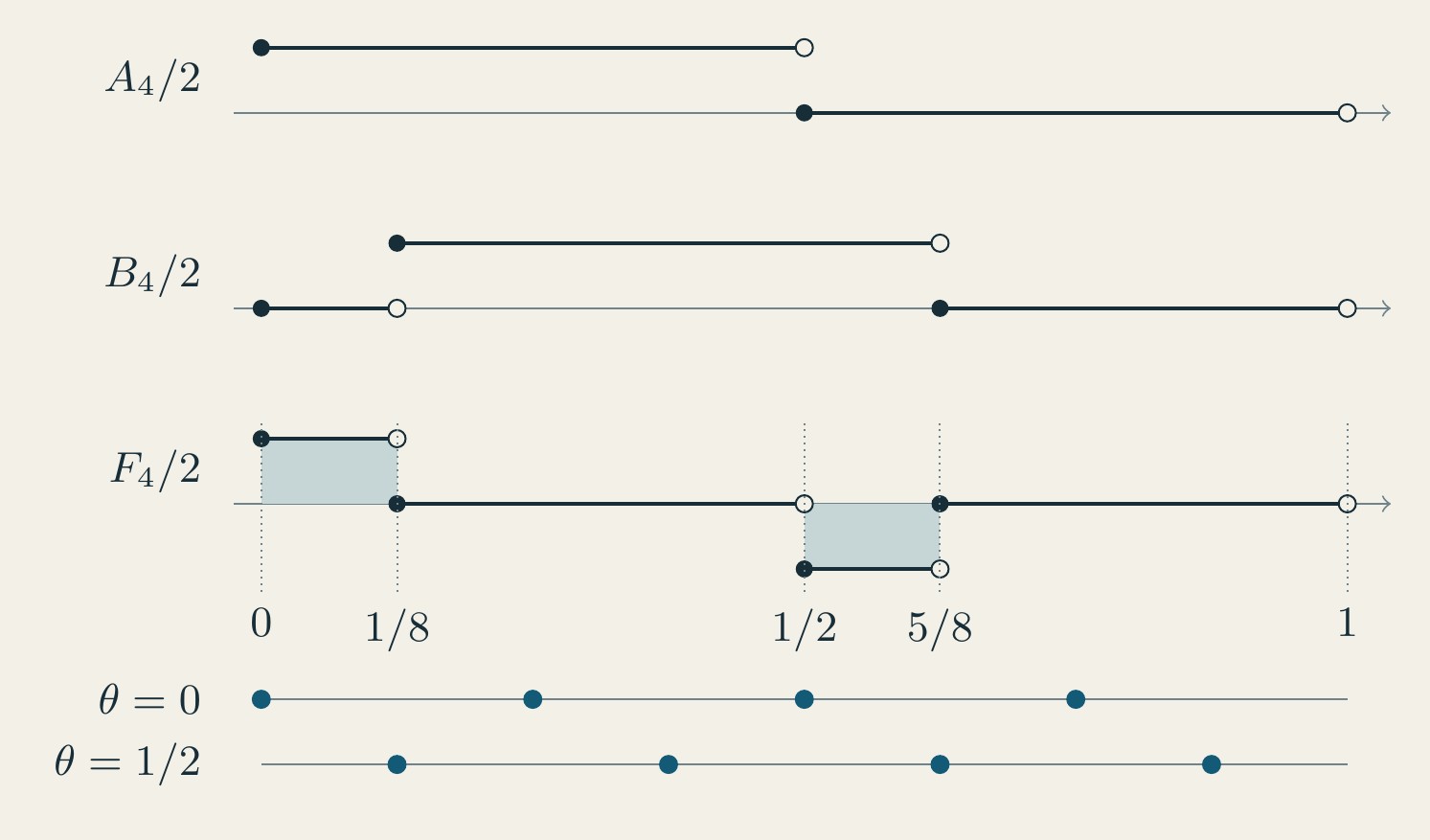
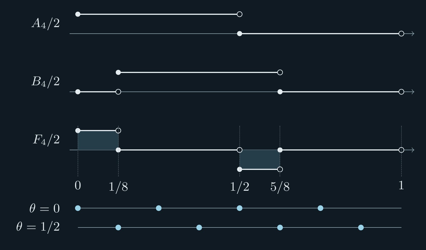
The curves are divided by two to show their shapes. Filled endpoints are included and open endpoints are excluded. The bottom two rows show sample locations. The unshifted grid meets the two nonzero pieces at their included left endpoints; the half-cell grid meets their excluded right endpoints.

The full calculation can be inspected in four readings.

Mixed-energy calculation.

Each gate has length $1/2$ and contains exactly $q/2$ grid samples, for every offset. Hence each channel has continuous and sampled energy $q/2$, and $D_{q,\theta}[A_q]=D_{q,\theta}[B_q]=0$. The continuous mixed energy is $$\int_0^1 A_qB_q\,dx=q(1/2-\delta_q)=q/2-1/2.$$ Their sampled mixed energy is the number of grid points in $[\delta_q,1/2)$. That number is $q/2-1$ when $\theta<1/2$ and $q/2$ when $\theta\ge1/2$. Therefore $$K_{q,\theta}(A_q,B_q)= \begin{cases}1/2,&0\le\theta<1/2,\\ -1/2,&1/2\le\theta<1, \end{cases} \qquad D_{q,\theta}[F_q]=-2K_{q,\theta}(A_q,B_q).$$ This recovers (35). Adding the two separate channel defects would give zero and lose the entire answer.

The combined-field and mixed-energy calculations give the same answer. The first locates the two short intervals; the second attributes the full defect to the interaction. The endpoint readings determine which grid offsets see that energy.

11.3. Method selection and extension

The last two problems ask for a choice of method and a transfer of the completed example. A solution should name the object that the chosen operation acts on before estimating it.

Part III. Finite arithmetic tools

Arithmetic data offer two useful ways to organize the preceding energy calculations. When components are specified by congruences, construct their observed intersections and use them as entries of a matrix. Sections 12 and 13 develop this route, including the effect of moving a boundary or changing the modulus of a phase.

When a kernel repeats under common dilation, group its repeated pairs into primitive shells. Sections 14 and 15 develop this second route. Logarithmic weighting connects the resulting prefixes to prime counting; recovering estimates from that identity requires control of its signed inverse. The two routes make arithmetic structure available to the field and observation calculations already established.

12. Signed collision registers

A congruence records where two arithmetic components can meet. An observation records which of those meetings are actually read. Keeping these two pieces of data together turns a collision count into a finite field to which the energy rules already apply.

Consider the two conditions $$r\equiv4\pmod7,\qquad r\equiv1\pmod8.$$ They have the common residue $25$ modulo $56$. An observation on $3<r<6$ sees no common reading; one on $24<r<27$ sees exactly one. Compatibility of the congruences is therefore only the first part of an interaction calculation. The interval and its weights determine whether that interaction contributes.

12.1. Incidences and the observation kernel

Let $\mathcal A$ be a finite set of arithmetic components. A component $\xi$ has modulus $c_\xi\ge1$, residue $\rho_\xi$, real amplitude $z_\xi$ and orientation $\sigma_\xi\in\{1,-1\}$. Define its incidence and the combined row by $$I_\xi(r)=\mathbf 1_{r\equiv\rho_\xi\;(\mathrm{mod}\;c_\xi)},\qquad \Delta(r)=\sum_{\xi\in\mathcal A}\sigma_\xi z_\xi I_\xi(r).$$ Give the integer rows nonnegative weights $v(r)$ of finite support. The energy and intersection kernel are $$M_v=\sum_r v(r)\Delta(r)^2,\qquad K_v(\xi,\eta)=\sum_r v(r)I_\xi(r)I_\eta(r).$$(36) Think of each component as a column and each address $r$ as a row. The entry $I_\xi(r)$ records whether that component is present there; its signed amplitude determines its contribution to the reading. Several columns can contribute to the same observed row. In this section $\Delta(r)$ names that combined reading; it is not the backward difference $\Delta h(n)$ used in the weighted identities.

This is the collision-matrix calculation of Section 8, with its entries evaluated by congruences. The matrix $K_v$ is positive semidefinite because it is a Gram matrix of incidence vectors. Its signed quadratic form nevertheless contains negative mixed terms. Replacing those terms by absolute values changes the energy being estimated.

12.2. Common residues and finite intervals

The Chinese remainder theorem supplies the common residue . Parentheses denote the greatest common divisor and brackets the least common multiple. Write $$g=(c_1,c_2),\qquad \ell=[c_1,c_2].$$ The notation $g\mid d$ means that $g$ divides $d$. A bar denotes an inverse in the displayed modulus. The two incidences meet exactly when $g\mid\rho_2-\rho_1$. If they meet, solve $$t\equiv\frac{\rho_2-\rho_1}{g}\, \overline{(c_1/g)}\pmod{c_2/g},\qquad R\equiv\rho_1+c_1t\pmod\ell,\quad 0\le R<\ell.$$ For $c_2/g=1$ take $t=0$. These formulas follow by substituting $r=\rho_1+c_1t$ into the second congruence. The reduced moduli are coprime, so the displayed inverse exists. Every common row is $R+j\ell$.

If the observation is supported on $Y<r<2Y$ and $\ell>Y$, there is at most one common row. Its first possible representative is $$j_0=\left\lfloor\frac{Y-R}{\ell}\right\rfloor+1,\qquad r_0=R+j_0\ell.$$ The kernel is $v(r_0)$ when compatibility holds and $r_0<2Y$; otherwise it is zero. The inequality $r_0>Y$ is already enforced. For a longer interval, retain the full sum $\sum_{j:\,Y<R+j\ell<2Y}v(R+j\ell)$.

12.3. A divisibility register

A useful arithmetic instance fixes an odd prime $p$ and uses moduli $p/2<c<p$ and columns $1\le b<p$. Put $$\Delta[f](r)=\sum_c a_c\sum_{1\le b<p}f_b \bigl(\mathbf 1_{c\mid p^2-br}-\mathbf 1_{c\mid p^2+br}\bigr), \qquad 1\le r<p,$$(38) where $a_c,f_b$ are real coefficients. The row weights $v(r)$ still specify the observation; $a_c$ and $f_b$ specify the field. A column $b$ is a unit modulo $c$ when $(b,c)=1$. Then its inverse $\bar b$ satisfies $b\bar b\equiv1\pmod c$. A unit component $(c,b,\sigma)$ has residue $\rho\equiv\sigma p^2\bar b\pmod c$. A nonunit $b$ has no incidence: any common divisor of $b,c$ would divide $p^2$, although $c<p$. For two unit components, compatibility becomes $$(c_1,c_2)\mid \sigma_1b_2-\sigma_2b_1.$$(39) Multiplying the common-residue condition by the unit $b_1b_2\overline{p^2}$ proves this equivalence. The interval test is still needed after (39).

Let $d_c(r)$ denote the $c$ term in (38). If $|a_c|\le A$, $|f_b|\le B$ and $\sum_r v(r)\le V$, then $$0\le\sum_r v(r)\sum_c d_c(r)^2\le16A^2B^2pV.$$(40) For fixed $c,r$ each sign permits at most two columns, since $c>p/2$. Hence $|d_c(r)|\le4AB$, and summing over fewer than $p$ moduli proves the bound. This retains all pairs at a common modulus, including distinct columns.

The remaining energy is the signed sum over different moduli. A first-moment target may require less than control of that energy: Cauchy–Schwarz gives $$\left|\sum_r W(r)\Delta(r)\right|^2 \le\left(\sum_r|W(r)|\right) \left(\sum_r|W(r)|\Delta(r)^2\right).$$ The implication goes from a second-moment bound to a first-moment bound. A row pair $T,-T$ has zero unweighted sum and energy $2T^2$, so the converse need not hold.

13. Boundary localization and reciprocal transfer

Moving the edge of a register changes only the columns crossed by that edge. The cost can be counted before any smooth approximation is chosen. For example, at $p=11,r=4$, changing column $b=10$ by $h$ changes (38) by $$h(a_9-a_7).$$ Indeed $p^2-br=81$ and $p^2+br=161$ have, respectively, the divisors $9$ and $7$ in $11/2<c<11$. The sign and the two modulus coefficients remain visible in the change.

13.1. Column budgets and energy transfer

Let $\tau(n)$ count the positive divisors of $n$.

The same change has a controlled effect on energy without dropping the inherited interaction. Set $h(r)=\Delta[f](r)-\Delta[g](r)$ and $M_v[f]=\sum_r v(r)\Delta[f](r)^2$. Then $$\begin{aligned} M_v[f]-M_v[g] &=2\sum_r v(r)\Delta[g](r)h(r)+\sum_r v(r)h(r)^2, \\ \left|\sqrt{M_v[f]}-\sqrt{M_v[g]}\right| &\le \|h\|_\infty\sqrt{\sum_r v(r)}.\notag \end{aligned}$$(42) The first formula is the field-change identity. The second is the reverse triangle inequality in the weighted square norm. Squaring a bound for $h$ alone would miss the first term in (42).

13.2. An adjustable smoothing width

Smoothing has two costs. A wider transition changes more columns; a narrower transition has larger derivatives. Both costs must refer to the same register.

Choose fixed smooth functions $\chi$ on $[0,1]$ and $u$ on the real line. Let $\chi$ vanish near zero, and let $u(t)=0$ for $t\le0$, $u(t)=1$ for $t\ge1$. For $1\le J\le p$ put $$f_b^\sharp=\chi(b/p),\qquad B^{[J]}(\beta)=\chi(\beta)u\bigl(p(1-\beta)/J\bigr).$$ Extend $B^{[J]}$ by zero outside $[0,1]$. The sharp and smooth tables differ only on $p-J<b<p$. Differentiation and a change of variable over an interval of length $J/p$ give $$\|(B^{[J]})'\|_1\le C,\qquad \|(B^{[J]})''\|_1\le Cp/J.$$(43) Here and below the profile constants are fixed.

Thus this hypothesis supplies normalized row size $O_\varepsilon(p^{-1/3+\varepsilon})$ after division by $p$. The proposition isolates the reusable step: choose the transition width after estimating its actual column cost. The smooth-row bound is an explicit additional input; it is not a consequence of the incidence identity. In the motivating short-variable calculation that input uses completion of exponential sums and a classical Weil bound. Its analytic proof is not needed to apply the budget principle to another family with its own smooth estimate.

The exponents also locate the limit of this particular calculation. Writing $J=p^\theta$ gives the two powers $\theta$ and $1-\theta/2$. Their maximum is least at $\theta=2/3$. Improving the exponent requires a better estimate for at least one cost or cancellation between the retained terms.

13.3. Reciprocal phase transfer

A smooth-row calculation may contain an inverse modulo a large modulus. A finite identity transfers that inverse to a smaller one and records the correction. Write $e(x)=\exp(2\pi i x)$.

For $r=4,c=7$, the relation $4\cdot2-7\cdot1=1$ gives $$e(2A/7)=e(-3A/4)e(A/28).$$ At $A=121$ the two phases are $242/7$ and $-363/4+121/28$; they differ by $121$, so their exponentials agree. The transferred inverse has modulus four. Its reciprocal correction $e(A/(rc))$ remains part of the field and may vary rapidly when $A$ grows. The identity changes coordinates; any cancellation estimate must still control the resulting amplitudes and phases.

14. Primitive shells and logarithmic transforms

Pairs $(1,2),(2,4),(3,6)$ have the same ratio. A kernel unchanged by common dilation assigns them the same reading. In a square cutoff $1\le a,b\le M$, the primitive pair $(1,2)$ appears $\lfloor M/2\rfloor$ times. Counting these repetitions is the starting point of a transform that separates primitive structure from its repeated observations.

In the arithmetic application, the kernel has a fixed modulus $q$, called its carrier modulus. The cutoff changes while $q$ stays fixed. This is the arithmetic counterpart of keeping a field fixed while changing its observation. The general decomposition below needs only invariance under common dilation.

14.1. Dilation-invariant kernels

Fix a maximum cutoff $M_0$. Let a real kernel $R(a,b)$ on $1\le a,b\le M_0$ satisfy $$R(da,db)=R(a,b)\qquad\text{whenever }d\max(a,b)\le M_0.$$ Define its square prefixes and primitive shells by $$\mathcal A(M)=\sum_{a,b\le M}R(a,b),\qquad P(m)=\sum_{\substack{\max(a,b)=m\\(a,b)=1}}R(a,b), \qquad \mathcal A(0)=0.$$(47)

The inversion uses the Möbius coefficient $\mu(r)$. For a positive integer $r$, $\mu(r)=0$ if a prime square divides $r$; otherwise $\mu(r)=(-1)^k$, where $k$ is its number of distinct prime factors, with $\mu(1)=1$. Thus $\mu(3)=-1$, $\mu(15)=1$ and $\mu(9)=0$.

The inversion is classical Möbius inversion . The useful choice in an application is the kernel whose common dilations really preserve the reading. Signed values are allowed throughout; no positivity or asymptotic hypothesis enters the proposition.

14.2. The logarithmic prefix operation

The factor $\lfloor M/m\rfloor$ counts every repetition of a primitive pair. A different weighting of those repetitions can select prime powers. The logarithmic operation below makes that change exactly, using the factorization identity for $\log n$.

Define the prime-power weight and its cumulative sum by $$\Lambda(n)= \begin{cases}\log\ell,&n=\ell^j,\ \ell\text{ prime},\ j\ge1,\\ 0,&\text{otherwise},\end{cases} \qquad \Psi(x)=\sum_{n\le x}\Lambda(n).$$ Empty sums are zero. Unique factorization gives $\log n=\sum_{d\mid n}\Lambda(d)$, so Möbius inversion gives $\Lambda(n)=-\sum_{d\mid n}\mu(d)\log d$. Summing over $n\le x$ yields the finite identity $$\Psi(x)=-\sum_{d\le x}\mu(d)\log d\left\lfloor x/d\right\rfloor.$$(50) These are the classical divisor identities for $\Lambda$ .

Apply the same coefficients to the square prefixes: $$\mathcal K(N)=-\sum_{d\le N}\mu(d)\log d\, \mathcal A(\lfloor N/d\rfloor).$$(51) The calligraphic letter distinguishes this prefix reading from the mixed defect $K_q(f,g)$ used earlier.

This theorem composes gcd grouping with classical convolution. It applies to any kernel satisfying the dilation hypothesis. Its usefulness depends on the resulting shell coefficients and the estimates available for the shorter prefixes.

14.3. A kernel supplied by clock boundaries

The midpoint sawtooth supplies such a kernel. Recall $\psi$ from Section 3, and put $$s(h,k)=\sum_{j=1}^{k-1}\psi(j/k)\psi(hj/k),\qquad s(h,1)=0.$$ Fix an odd prime $p$, let $q=p^2$, and restrict all indices to $1\le a,b<p$. Define $$R_q(a,b)=s(a\bar q,b)+s(b\bar q,a).$$(53) Every inverse uses the denominator of its own sum. The carrier $q$ stays fixed in $\mathcal A_q(M)$, $P_q(m)$ and $\mathcal K_q(N)$.

Here is the connection to the boundary calculus. For $f_a(x)=2\psi(ax)$, $$K_{q,0}(f_a,f_b) =\frac1q-\frac{a/b+b/a}{3q^2}+\frac4qR_q(a,b).$$(54) To verify it first take $(a,b)=1$. The product $f_af_b$ has point correction one at zero and no other sampled boundary. At $j/a$, $1\le j<a$, its value jump is $-4\psi(bj/a)$; the other clock gives the symmetric terms. Their boundary sum is $$\frac4q\sum_{j=1}^{a-1}\psi(bj/a)\psi(qj/a) +\frac4q\sum_{j=1}^{b-1}\psi(aj/b)\psi(qj/b) =\frac4qR_q(a,b),$$ after permuting residues by $q$. The slope-jump contributions, including the origin, are $-2q^{-2}(b/(6a)+a/(6b))$. This uses $\sum_{j=0}^{a-1}\widetilde B_2(qj/a)=1/(6a)$. The regular curvature is the constant $8ab$ and has zero Bernoulli integral. Theorem 4.1 now gives (54).

For a common divisor $d=(a,b)$, remove $d$ from both clocks. Integer dilation preserves their continuous pairing and permutes the $q$-grid, since $(d,q)=1$. It also preserves the kernel: $$s(dh,dk)=s(h,k).$$ Indeed, group the summation index by its residue modulo $k$ and use $$\sum_{j=0}^{d-1}\psi((x+j)/d)=\psi(x).$$ Inverses of $q$ reduce consistently to smaller denominators. This proves both the general pair formula and the common-dilation hypothesis for $R_q$.

Thus primitive-shell grouping applies to the signed remainder already produced by the boundary decomposition. The classical Dedekind sum provides a compact notation for its boundary phases.

14.4. A finite prime-counting example

For $m>1$, pair the two orientations of a primitive collision. The unit residues in the second Dedekind term cancel under $k\mapsto m-k$, giving $$P_q(m)=2\sum_{\substack{1\le k<m\\(k,m)=1}}s(m\bar q,k).$$(55) Also $P_q(1)=0$. Directly from the defining sums, $$s(1,2)=0,\qquad s(1,3)=\frac1{18},\qquad s(2,3)=-\frac1{18},\qquad s(1,4)=\frac18.$$ Because $p^2\equiv1\pmod{12}$ for primes $p\ge5$, these give $$P_q(1)=P_q(2)=P_q(3)=0,\qquad P_q(4)=\frac19,\qquad P_q(5)=\frac5{36},$$(56) with the last coefficient used when $p\ge7$. For $m=4$ only $k=3$ contributes; for $m=5$ the nonzero terms are $k=3,4$.

Take $q=121$ and $N=10$. In (52), the first three shells vanish and all $m\ge6$ have $10/m<2$, so $$\mathcal K_{121}(10) =\left(\frac19+\frac5{36}\right)\log2=\frac14\log2.$$ This is a complete example of prime counting inside a transformed collision reading.

Primitive means coprime coordinates, not a prime shell index. For instance (55) gives $P_{49}(6)=-2/5$ and $P_{121}(6)=2/5$, whereas $\Lambda(6)=0$. The shell keeps its carrier dependence and signs. Those features matter when the identity is used for estimates.

15. Prescribed fields and quantitative recovery

An identity specifies the quantity to be estimated. Replacing it by a bound for every possible field can impose a much stronger requirement. For the matrix $\operatorname{diag}(T,-T)$, the vector $(1,1)$ has quadratic reading zero although the operator norm is $|T|$. Large directions need not be the direction selected by the problem.

The distinction has an arithmetic instance in the kernel just constructed. It also appears when an exact inverse formula is used to recover individual prime-counting errors.

15.1. An interior operator-norm obstruction

Let $H=\lfloor\sqrt p\rfloor$ and choose real weights $0\le w_a\le1$ that equal one on $H\le a\le p-H$. These weights modify the kernel coefficients; they are distinct from the row masses of a register. Form the symmetric matrix $$R_w=(w_aw_bR_q(a,b))_{1\le a,b<p}.$$ Its prescribed scalar reading is $\mathbf1^TR_w\mathbf1=\sum_{a,b<p}w_aw_bR_q(a,b)$. Let $\Pi$ be orthogonal projection perpendicular to the constant vector. Removing that direction still leaves a large norm.

Thus a uniform $O_\varepsilon(p^{1/2+\varepsilon})$ norm bound, for every $\varepsilon>0$, is unavailable even on the mean-zero subspace. This does not decide the prescribed scalar sum. The lesson is to retain the source vector when choosing an estimate: an operator bound must pay for directions that the scalar may never use.

15.2. Exact recovery and stability

The logarithmic transform has a different issue. It can reconstruct a quantity exactly while enlarging a termwise error allowance. Keep the carrier $q=p^2$ fixed. Since the first nonzero shell is $P_q(4)=1/9$, the prime-counting identity at $N=4n<p$ gives $$\Psi(n)=9\mathcal K_q(4n) -9\sum_{m=5}^{4n}P_q(m)\Psi(4n/m).$$(58) For integer $n\ge2$, every argument on the right has integer part less than $n$. The initial prime count is $\Psi(x)=0$ for $x<2$. Hence the formula is a finite triangular recovery, despite $P_q(1)=0$ preventing an ordinary Dirichlet inverse.

To examine errors, retain the complete linear term: $$F_q(N)=\mathcal K_q(N)-N\sum_{m\le N}\frac{P_q(m)}m,\qquad E(x)=\Psi(x)-x.$$ Subtracting that term from (52) gives $$\begin{aligned} F_q(N)&=\sum_{m\le N}P_q(m)E(N/m), \\ E(n)&=9F_q(4n)-9\sum_{m=5}^{4n}P_q(m)E(4n/m). \end{aligned}$$(59, 60) These formulas include arguments between one and two, where $E(x)=-x$.

Suppose an induction tries to propagate the allowance $|E(x)|\le Cx^\alpha$ by taking absolute values in (60). The $m=5$ term alone has coefficient $$9|P_q(5)|(4/5)^\alpha =\frac54(4/5)^\alpha=(5/4)^{1-\alpha}.$$(61) For $\alpha<1$ this exceeds one. At square-root scale it is $\sqrt5/2$. Thus that absolute induction does not contract. The signed recurrence remains intact; the calculation identifies the information discarded by the attempted estimate.

15.3. Additional estimates for the arithmetic application

The transform uses shorter prefixes at the same carrier. At $N=p-1$, the coefficient of $d=1$ in (51) vanishes because $\log1=0$. Every remaining prefix therefore has cutoff at most $(p-1)/2$. A bound on $\mathcal A_{p^2}(p-1)$ alone supplies neither those readings nor their logarithmically weighted sum. Replacing $p$ by a smaller prime also changes the kernel.

A quantitative prime-distribution application needs estimates for these fixed-carrier prefixes and control of the signed recovery in (60). Those estimates are open for the collision family considered here. The proved tools are the finite decomposition, the transform and the recovery identity. Their use has made the missing information explicit.

The same discipline applies to the register moment. Its finite pair formula retains all signs and observed intersections; an improved rate requires an estimate for their joined sum. The smoothing proposition gives the stated one-third normalized rate under its explicit analytic hypothesis. It supplies no stronger rate merely by changing the width.

Part IV. Arithmetic energy at growing scales

The preceding parts give operations for an exact finite account. A growing arithmetic field also requires control of the dependence on scale. The two applications here make that dependence concrete.

Carry tables supply a periodic clock field. Moving its sampling grid changes the simultaneous boundary readings, and the half-cell calculation follows that change through to a limit. Tapered divisor families change both their source and their activation cutoff. Completed-cycle screening controls part of their interaction; the whole-field calculation retains the remaining tail, parent shell and combined resets. Local invariant readings then measure energy that later additions must leave behind.

16. Carry tables and clock families

In base three, the equal-digit words $00,11,22$ have numerical values $0,4,8$. They pick out three positions among the nine possible two-digit words. More generally, a repeated digit $dd$ in base $p$ has value $(p+1)d$. The carry count defined below tests these selected positions at each integer address $a$. A floor difference counts the integers crossed between $na/q$ and $(n+1)a/q$. Centering removes the term $a/p$ so that the remaining fluctuation can be compared with a clock field.

Let $p$ be an odd prime, $N=p-1$ and $q=p^2$. The equal-digit base-$p$ words occupy the positions $G_p=\{(p+1)d:0\le d<p\}$ on a circle of $q$ positions. Their carry count and centered reading are $$C_p(a)=\sum_{n\in G_p} \left(\left\lfloor\frac{(n+1)a}{q}\right\rfloor -\left\lfloor\frac{na}{q}\right\rfloor\right),\qquad F_p(a)=C_p(a)-\frac ap.$$ Write $E_p=\sum_{a=0}^{q-1}F_p(a)^2$ and $B_N(x)=2\sum_{j=1}^N\psi(jx)$. For $p=3$ and $a=1$, the three floor differences are $0,0,1$, so $C_3(1)=1$ and $F_3(1)=2/3$. The next lemma identifies every centered table reading with a reading of $B_2$, after permuting the nine addresses. It therefore transfers the entire squared table, not just its average, to the clock calculation.

At a reduced boundary $a/k$, the clocks whose frequencies are multiples of $k$ reset together. There are $\lfloor N/k\rfloor$ of them. Grouping the other frequencies into blocks of length $k$ cancels each complete block; only the final incomplete block contributes to the inherited reading. The next notation records the number of complete blocks, the remaining length and that remaining reading. Each reduced fraction is counted once by requiring $a$ and $k$ to be coprime.

For $2\le k\le N$, set $$M_k=\lfloor N/k\rfloor,\quad s_k=N-kM_k,\quad T_{k,s}(a)=2\sum_{j=1}^s\psi(ja/k),\quad H_N=\sum_{j=1}^N\frac1j.$$ Let $\mathcal U_k=\{1\le a<k:(a,k)=1\}$, and put $$\mathcal A_p=\sum_{k=2}^NM_k \sum_{a\in\mathcal U_k}T_{k,s_k}(a)\psi(p^2a/k).$$

The continuous energy can also be read from pairwise clock collisions. The Fourier coefficients of $\psi$ are $-1/(2\pi i n)$ for $n\ne0$. The frequencies common to $\psi(jx)$ and $\psi(kx)$ give, by Parseval, $$\int_0^1\psi(jx)\psi(kx)\,dx=\frac{(j,k)^2}{12jk},\qquad \int_0^1B_N^2\,dx=\frac13\sum_{j,k\le N}\frac{(j,k)^2}{jk}.$$ Together with Lemma 16.1, this recovers both sides of the carry-energy comparison from the same finite family.

For $p=3$, $\mathcal A_3=0$ and $H_2=3/2$, giving $D_9[B_2]=4/9-1/27=11/27$. In general, the established unit-sampling theorem for this carry family [5] supplies the separate estimate $$D_{p^2}[B_{p-1}] =1+O\!\left(p^{-1/458696}\log^4(2p)\right).$$ Equation (62) identifies its residual as $4\mathcal A_p/p^2-NH_N/(3p^3)$. The boundary decomposition does not replace the signed estimate proving that this residual tends to zero. The finite common-reset contribution is $(p-1)^2/p^2$.

17. Half-cell carry grids

At the origin all $p-1$ clocks reset together. A half-cell shift misses that point and samples the reset at one half, where only the even-frequency clocks reset. The number of resetting clocks is halved, so their squared amplitude is quartered. This identifies the candidate change in the limit. The rest of the section calculates the other boundary terms and controls their combined contribution.

Retain the field $B_N$, with $N=p-1$, but sample it at $(a+1/2)/p^2$. This changes the sampling rule while leaving the continuous energy fixed. It is a shifted observation of the clock field; no new interpretation of these points as integer carry inputs is required.

Put $M=N/2$ and define the shifted interior source $$\mathcal A_p^{\rm half} =\sum_{k=2}^NM_k\sum_{a\in\mathcal U_k} T_{k,s_k}(a)\psi(p^2a/k-1/2).$$ The location $1/2$ is now sampled. Exactly the even-frequency clocks reset there. All the odd-frequency clocks have reading zero there as well, since $\psi(j/2)=0$ for odd $j$. Consequently $C_{1/2}=M$, $U_{1/2}=0$, and $B_N(1/2)=0$.

For $p=3$ the nine readings on the half-cell grid are $$-\frac53,\ -1,\ -\frac13,\ \frac13,\ 0,\ -\frac13,\ \frac13,\ 1,\ \frac53.$$ Their squares sum to eight. The continuous energy is one, so the defect is $1-8/9=1/9$, agreeing with the boundary calculation. In this example both the shifted interior source and the harmonic correction vanish.

17.1. Residual criterion

The point correction satisfies $$\frac{M^2}{p^2}=\frac{(p-1)^2}{4p^2}\longrightarrow\frac14,$$ and the harmonic term is $O(p^{-2}\log(2p))$. As $p$ tends to infinity through odd primes, $$D_{p^2,1/2}[B_{p-1}]\longrightarrow\frac14 \quad\Longleftrightarrow\quad \mathcal A_p^{\rm half}=o(p^2).$$(64) This equivalence distinguishes a limit for the sampled collision amplitude from a limit for the complete energy defect.

To compare the new source with the unshifted one, define for positive integers $N,Q$ $$\mathcal A_N(Q)=\sum_{k=2}^N\lfloor N/k\rfloor \sum_{a\in\mathcal U_k}T_{k,N\bmod k}(a)\psi(Qa/k).$$ There is no coprimality hypothesis in this definition. The original source is $\mathcal A_p=\mathcal A_{p-1}(p^2)$.

The same shift also has a direct grid interpretation: $$D_{q,1/2}[B_N]=2D_{2q}[B_N]-D_q[B_N].$$ It follows from (12). This relation is exact for each fixed $N$. It does not supply an estimate for $D_{2q}$ along the growing family.

17.2. Parity-restricted source

The unshifted estimate controls $\mathcal A_N(q)$ for $N=p-1$, $q=p^2$. Its count-source transformation uses the inverse of $q$ modulo every $l\le N$. The replacement $q\mapsto2q$ is not permitted at even moduli. For instance, multiplication by $25$ permutes the residues modulo four, while multiplication by $50$ reaches only the even residues. An inverse exists for the first map and not for the second. Formula (67) removes that algebraic obstruction, and leaves three parity-restricted sums. Their cancellation can be transferred by retaining parity through the full reciprocity descent.

Recall the Dedekind sum from Section 14. Since $\psi(0)=0$, its equivalent form with the zero term included is $s(h,k)=\sum_{a=0}^{k-1}\psi(a/k)\psi(ha/k)$, with $s(h,1)=0$. The argument $h$ need not be a unit. At odd $l$, $2q$ is invertible; at every $k\le M$, $q$ is invertible. Hence the remaining source is exactly $$\begin{aligned} \mathcal A_N(2q) ={}&2\sum_{\substack{l\le N\\l\ {\rm odd}}} \sum_{j=1}^N s(j\overline{2q},l)\\ &+4\sum_{k=1}^M\sum_{r=1}^M s(r\bar q,k) +2\sum_{k=1}^M\sum_{r=1}^M s((2r-1)\bar q,k).\notag \end{aligned}$$(68) The modulus-one terms are understood as zero. The bars denote inverses in the modulus of their summand. This formula follows by splitting (66) into odd and even $l$ and then using (67).

The finite identities above identify the new source created by the shift. The next lemma supplies the additional analytic transfer needed for its limit. The unit-limit theorem alone does not supply this step. Readers interested first in using the calculus may continue at Theorem 17.4 and its interpretation, then return to the transfer proof with the cited analytic source available.

17.3. Parity transfer

Parity restricts the source to a fixed number of arithmetic progressions in the reciprocity calculation. The following estimate makes that transfer explicit. Its analytic ingredients are the reciprocal-phase, completion and stopped-descent estimates in .

The two cutoff variables $X,Y$ describe a rectangle of indices, allowing its sides to end at different places. Uniformity in both matters because splitting into even and odd indices changes those endpoints. The proof first converts clock correlations into modular interval counts. Finite Fourier sums retain the restriction to odd indices while completing the counts to whole residue systems. Reciprocity then reduces the modular pairs to smaller ones; the restriction is followed through that reduction. The required saving is below $p^2$. Once divided by the sampling scale $p^2$, the bound in the lemma tends to zero.

The grid shift changes which combined reset is sampled. Its surviving amplitude falls from $N$ to $N/2$. The two limits, one and one quarter, record the square of that change after the interior source has been estimated. The boundary calculation identifies the limit’s contribution; the parity transfer controls everything that remains.

17.4. Finite readings of the shifted field

The boundary term and the full defect approach their limits in different ways. The following values separate the sampled point contribution $M^2/p^2$ from the signed source $4\mathcal A_p^{\rm half}/p^2$. They are rounded displays of rational calculations made with nfield [8], software for exact arithmetic calculations.

Each row can be reconstructed by evaluating $B_N$ at the $p^2$ half-cell sample points, averaging their squares, and subtracting that average from the continuous Gram sum in Section 16. The boundary formula (63) gives an independent calculation of the same defect.

The sampled point correction increases toward one quarter. The full defect fluctuates on both sides of that value in the displayed range. For example, the boundary contributions at $p=53$ and $p=97$ are already close, but their signed sources have opposite signs. The table makes the role of the residual visible. Its uniform decay, proved in Theorem 17.4, establishes the limit.

18. Completed cycles and weighted interaction

A field built from many periodic families presents two different scales. An old family may have completed its source profile and repeat with zero mean, while a new family is still changing. Their interaction is controlled by the old primitive and the variation of its weighted partner.

This section constructs one such field and applies the weighted rules of Section 9. The single-family estimate retains the length of the old cycle. Summing it then determines how many families can be controlled together. That distinction between one interaction and the whole field is the central calculation.

18.1. Tapered divisor families

Each odd label $r$ starts a family at length $r$ and follows it through $2r,4r,8r$. The profile assigns the signed levels on those successive bands. The taper $\tau_S$ keeps the profile unchanged through $S$, reduces it linearly to zero at $2S$, and vanishes beyond that point. Multiplying the tapered profile’s first difference at $j$ by $j$ produces the clock coefficients. This order matters at every band boundary and at $2S$.

Completed old profiles have zero period mean. Their changing weighted partners make this a test of the primitive estimate for a whole family of interactions.

The families are joined with the Möbius coefficients introduced in Section 14. Their signs remain in the combined field before it is squared. The same divisor-inversion identity will later connect the family source to its reset readings.

The family profiles below specify the complete source, including its taper and terminal coefficients. Their size, reset variation and screening bounds follow from these definitions. Let $t\ge1$ be an integer, $S=4t$, and $$\tau_S(j)=\min(1,\max(0,(2S-j)/S)).$$ For each positive odd core $r$, write its profile as $$\phi_r(j)=\frac1r\left( \mathbf 1_{\{r\le j<2r\}}-\mathbf 1_{\{2r\le j<4r\}} +\frac14\mathbf 1_{\{4r\le j<8r\}}\right).$$ Define the family source, raw field and joined source by $$\begin{gathered} q_{t,r}(j)=j\Delta[\tau_S(j)\phi_r(j)],\qquad f_{t,r}(n)=\sum_jq_{t,r}(j)\{n/j\},\\ q_t(j)=\sum_{r\ {\rm odd}}\mu(r)q_{t,r}(j),\qquad p_t(n)=\sum_{r\ {\rm odd}}\mu(r)f_{t,r}(n),\qquad B_t=E_S[p_t]. \end{gathered}$$ Only $r<2S$ occur in the parent, and every source includes its terminal coefficient at $j=2S$. These are the prescribed Möbius families. Indeed, with $A(x)=\sum_{d\le x}\mu(d)/d$, $$A(j)-\frac32A(j/2)+\frac12A(j/4) =\sum_{r\ {\rm odd}}\mu(r)\phi_r(j).$$ This follows by separating odd $d$ and $d=2r$ in $A$; terms divisible by four have zero Möbius coefficient. Denoting the left side by $F(j)$ gives the original source $q_t(j)=j\Delta[\tau_S F](j)$. In particular $q_t(1)=1$ is retained, and $\sum_jq_{t,r}(j)/j=\sum_jq_t(j)/j=0$ by telescoping. The real-address fields are constant on open unit cells, so their continuous native integral in (18) uses exactly those clock readings.

At doubling put $\delta f_r=f_{2t,r}-f_{t,r}$ and $\delta p=p_{2t}-p_t$. Only $S/8<r<4S$ can change. If $8m\le S$, the complete old family is unchanged and equals $$H_m(n)=\{n/m\}-4\{n/(2m)\}+5\{n/(4m)\}-2\{n/(8m)\}.$$ Its eight-block profile is $$H_m(n)=h(\lfloor n/m\rfloor\bmod8),\qquad h=(0,-1,2,1,-1,-2,1,0).$$

18.2. Completed-cycle screening

A completed old family repeats with zero mean. Against a constant partner, each complete period contributes zero. A changing weighted partner leaves work controlled by its variation, just as the alternating four-term example did in Section 7. Here the period has length $8m$, so the primitive bound must retain its dependence on $m$. That dependence determines how many families the estimate can control.

The completed profile has zero period mean and $|H_m|\le2$. Its primitive $F_m(N)=\sum_{n=1}^NH_m(n)$ stays between $-m$ and $2m$. To see this, the values at block ends $N=jm-1$, $j=1,\ldots,8$, are $0,-m,m,2m,m,-m,0,0$. Between block ends the increments have constant sign, and complete periods sum to zero. Subtracting two primitive values consequently gives $$\left|\sum_{n=a}^bH_m(n)\right|\le3m\qquad(1\le a\le b).$$(75)

The bound uses a small primitive of the old field, not a universal sign of its interaction. The infinite tail and the actual jumps of its partner remain present throughout.

18.3. Summed screening bound

For an integer $0\le M\le S/8$, define the short old field and its work $$p_{\le M}(n)=\sum_{\substack{m\le M\\m\ {\rm odd}}}\mu(m)H_m(n), \qquad W_S(M)=2\sum_{n>2S}w_np_{\le M}(n)\delta p(n).$$ The core sums are finite and the native products are absolutely summable, so $$W_S(M)=2\sum_{\substack{m\le M\\m\ {\rm odd}}} \sum_{\substack{S/8<r<4S\\r\ {\rm odd}}} \mu(m)\mu(r)K_S(m,r).$$ There are at most $2S$ changed odd labels. Since the odd positive integers through $M$ sum to $\lceil M/2\rceil^2$, the theorem gives $$|W_S(M)|\le\frac{516}{S}\lceil M/2\rceil^2 \le129\frac{(M+1)^2}{S}.$$(77) For $$M_S=\min(\lfloor S/8\rfloor,\lfloor\sqrt S\rfloor)$$ this is at most $516$. It controls the interaction of all those short old cycles with every changed family. No cancellation among their Möbius signs is required for this portion.

The same proved estimate also allows a logarithmically longer range. With $\ell_t=1+\lfloor\log_2t\rfloor$, take $$M_t^\star=\min\bigl(\lfloor S/8\rfloor, \lfloor\sqrt{S\ell_t^3}\rfloor\bigr).$$ Then (77) gives $|W_S(M_t^\star)|\le516\ell_t^3$. This controls the complete work against every changed family through that cutoff. A range $S^{1/2+\epsilon}$ for fixed $\epsilon>0$ would require a further saving.

Taking $M=\lfloor S/8\rfloor$ in the same bound instead gives $O(S)$. The number and total cycle scale of the old families consume the saving in the pair estimate. This is an upper allowance from that estimate, not a lower bound on the actual signed work.

18.4. Finite evaluation of an infinite interaction

The screening bound concerns the complete series. A finite calculation can approximate it with an explicit error. For $N\ge2S$ set $$K_{S,N}(m,r)=\sum_{2S<n\le N}w_nH_m(n)\delta f_r(n).$$ The bounds $|H_m|\le2$ and $|\delta f_r|\le12$ give $$|K_S(m,r)-K_{S,N}(m,r)| \le24\sum_{n>N}\frac1{n(n+1)}=\frac{24}{N+1}.$$ Thus the finite rational sum specifies an interval containing the infinite interaction. Taking $N\ge2399$ makes its half-width at most $1/100$; a valid cutoff must also satisfy $N\ge2S$. The calculation requires the actual fractional-clock readings at each integer, including resets. An equivalent evaluation uses the neutral floor sum from Section 9.

The finite interval and the all-scale theorem answer different questions. The interval encloses one chosen interaction; the screening theorem controls every admissible pair with its stated dependence on $m,S$.

18.5. Large primitives and the screening bound

Joining the old families before estimating gives a more informative version of the same method. Put $$F_M(n)=\sum_{\substack{m\le M\\m\ {\rm odd}}}\mu(m)F_m(n), \qquad J_{S,M}=\sup_{n\ge2S}|F_M(n)-F_M(2S)|.$$ The weighted variation of the complete changed field is at most $86/S$. Indeed there are at most $2S$ changed labels, and the proof of Theorem 18.2 bounds each weighted variation bracket by $43/S^2$. Therefore $$|W_S(M)|\le172J_{S,M}/S.$$(78) The signs have now entered $F_M$. They do not, however, make this primitive uniformly small at every address.

For $M$ of order $S^{1/2+\epsilon}$, any fixed $\epsilon>0$, the uniform primitive estimate required to make (78) logarithmic is therefore false. The large readings may occur at very distant addresses. Their existence does not give a large native weighted interaction, because those addresses have small masses. A useful refinement must retain the weighted location of the primitive and its correlation with the changed source.

19. Native energy under refinement

At a doubled scale, both the clock field and its activation cutoff change. The observed energy loses the parent shell and gains the child field on the common tail. The field-change identity of Section 9 determines the whole increment before any families are separated.

Retain the fields of Section 18, with $S=4t$ and $B_t=E_S[p_t]$. We first localize the full increment to a finite interval with a controlled tail. Aligning completed cycles then exposes the parent-shell credit, and combining resets gives a finite formula for the remaining work. Each step preserves the same energy change.

19.1. Complete energy change

Put $p_>=p_t-p_{\le M_S}$. The full moving-field identity is $$\begin{aligned} B_{2t}-B_t&=W_S(M_S)+R_S^{\rm nat},\\ R_S^{\rm nat} &=-\sum_{S<n\le2S}w_np_t(n)^2\notag\\ &\quad+\sum_{n>2S}w_n \bigl(2p_>(n)\delta p(n)+\delta p(n)^2\bigr). \notag \end{aligned}$$(79) The negative parent shell has not been split. The common tail includes all interactions with the remaining old cores and every interaction between changed cores. In particular $p_>$ contains intermediate completed cycles as well as families near the moving cutoff.

Write $\ell_t=1+\lfloor\log_2t\rfloor$ for the number of doubling scales through $t$. It will measure the desired growth allowance.

19.2. Finite localization of native work

The weight of an address now supplies an effective limit on how far large primitive readings can matter. There are at most $S$ odd labels in the parent and $2S$ in the child. Lemma 18.1 therefore gives, at every integer address, $$|p_t(n)|\le6S,\qquad |p_{2t}(n)|\le12S.$$ These bounds are coarse in amplitude but useful in the distant tail.

The infinite tail has now been accounted for by an absolute allowance. The remaining arithmetic estimate concerns the finite addresses $S<n\le S^2$. A large primitive reading obtained by a distant congruence construction need not occur inside this interval. Localization retains that distinction without requiring a uniform bound on the primitive over all addresses.

19.3. Cycle alignment and parent credit

The common start at $2S$ can cut an old cycle in the middle. Moving that family’s start back to its previous period boundary makes its primitive start at zero. But the move restores readings between the two starts. Those fragments all lie in the parent shell already removed by the activation change. Their combined field $Z_S$ must therefore be accounted for together with the old shell field. The construction below keeps that adjustment as a signed difference of two whole squares.

Here take $M=\lfloor S/8\rfloor$, so every completed old family is included. The earlier cutoff $M_S$ selected only the sufficiently short cycles controlled by screening. The alignment below is an identity for the larger range; estimating its signed work remains a separate task. Put $Y=\delta p$ and define $$\begin{gathered} L_m=8m\left\lfloor\frac{2S}{8m}\right\rfloor,\qquad Z_S(n)=\sum_{\substack{m\le M\\m\ {\rm odd}}} \mu(m)H_m(n)\mathbf 1_{\{L_m<n\le2S\}},\\ C_M=p_{\le M},\qquad P_>=p_t-C_M,\\ \widetilde W_S= 2\sum_{\substack{m\le M\\m\ {\rm odd}}}\mu(m) \sum_{n>L_m}w_nH_m(n)Y(n). \end{gathered}$$ Since $8m\le S$, one has $S<L_m\le2S$. Every restored fragment lies inside the same removed parent shell.

The fragment diagonal is paid uniformly. The joined fragment square also contains all interactions between distinct families, so $D_Z$ cannot replace $\sum w_nZ_S(n)^2$. The useful quantity in the identity is the signed difference $T_S$ itself.

For the aligned work the primitive $F_m$ vanishes at $L_m$. The full infinite summation-by-parts identity is $$\begin{aligned} \sum_{n>L_m}w_nH_m(n)Y(n) ={}&\sum_{n>L_m}F_m(n)(w_n-w_{n+1})Y(n)\\ &+\sum_j\delta q(j) \sum_{j\ell\ge L_m+2}w_{j\ell}F_m(j\ell-1). \end{aligned}$$ At a finite upper endpoint $N$, the first sum stops at $N-1$, the reset sum at $j\ell\le N$, and $F_m(N)w_NY(N)$ must be added. The endpoint vanishes as $N\to\infty$. Weight variation is summable, and each of the finitely many reset progressions has summable weights. This justifies the displayed limit. Moving the initial boundary changes the reset cutoff as well as the primitive’s initial value.

19.4. Parent-shell response

On the removed shell the actual divisor identity gives a shorter formula for the parent field. Retain the notation $F(n)=A(n)-\tfrac32A(n/2)+\tfrac12A(n/4)$.

This is a consequence of the prescribed Möbius source. Replacing its family coefficients arbitrarily would remove the divisor identity on which the proof depends. The formula evaluates the negative shell in (80); that shell remains the square of the whole parent field.

The first-shell formula evaluates the parent at every admitted address, including those at which restored cycle fragments are active. In the cycle credit, the later retained-field square contributes to the same account as the early shell. Keeping both joined squares preserves the signed difference in (82).

19.5. Joined resets on doubling blocks

After localization, the remaining task is a finite sum of energy changes. Grouping addresses into doubling blocks makes it possible to compare the sizes of contributions at different distances. The boundary at the end of one block is the start of the next, so its endpoint term must cancel when the blocks are rejoined. Within a block we keep the combined reset amplitude and its interaction with the preceding field.

The finite interval can be partitioned at $2S,4S,8S,\ldots$, ending with $S^2$. To evaluate its work by resets, combine the clocks that reset at the same address. Define $$a(n)=\sum_{\substack{j\mid n\\j\le2S}}q_t(j),\qquad d(n)=\sum_{\substack{j\mid n\\j\le4S}}\delta q(j),\qquad g(n)=p_{2t}(n)^2-p_t(n)^2.$$ The source has been extended by zero outside its support. Reciprocal neutrality gives $\Delta p_t(n)=-a(n)$ and $\Delta Y(n)=-d(n)$.

No intermediate block endpoint has acquired a separate charge. Formula (84) also retains interactions between distinct divisors at the same address. Splitting $a$ and $d$ into individual clock magnitudes would lose those signs.

The immediate envelope estimate on a block is $$\sum_{u<n\le v}w_ng(n) \le144S^2\left(\frac1{u+1}-\frac1{v+1}\right).$$ Its sum from $2S$ to $S^2$ is of order $S$. Thus localization and regrouping have identified a finite signed target, but the desired logarithmic estimate still requires a bound for the actual correlations in (84). The parent shell and all block signs remain available together in (86).

19.6. Uniform increment estimate

With $\ell_t=1+\lfloor\log_2t\rfloor$, the remaining estimate is $$\boxed{R_{4t}^{\rm nat}\le C\ell_t^3\qquad(t\ge1).}$$(87) Since $|W_S(M_S)|\le516$, this estimate is equivalent, up to a changed absolute constant, to $B_{2t}-B_t\le C'\ell_t^3$. The estimate is open. Summing it along a doubling chain would give a fourth-power logarithmic energy bound; that energy bound alone would not control each increment.

Uniform control must account for the changing field. Fixed-field quadrature constants depend on its boundary data and curvature norms. The half-cell parity transfer addresses another field and observation; it does not bound the native remainder in (79).

20. Invariant readings on the parent shell

The parent-shell credit contains a negative retained-field square. A lower bound for that square can therefore give an upper bound for the energy change. This applies the invariant-reading method of Section 8 to a concrete family of allowed additions.

The later families vanish on the inherited prefix. On the parent shell, their first nonzero readings form a triangular matrix. That structure lets us construct local invariants and compare the information they retain with the full constrained minimum. A finite counterexample will show exactly what a sparse collection of readings can miss.

20.1. Four-reading invariants

The retained field in the parent credit is $p_t-Z_S$. The inherited prefix fixes the coefficients of the old families. Indeed, at an odd address $m\le S$ the untapered reset amplitude is $\sum_{r\mid m}c_r$. The prescribed prefix makes it one at $m=1$ and zero at all other odd $m\le S$; divisor inversion gives $c_r=\mu(r)$ for odd $r\le S$. Every odd family with $S<r<2S$ vanishes through address $S$. These later families have a particularly simple response on the shell $I_S=\{S+1,\ldots,2S\}$. The following construction develops the invariant readings fixed by that prefix.

Write the inherited retained field and an arbitrary later addition as $$v_S=\sum_{\substack{r\le S\\r\ {\rm odd}}}\mu(r)f_{t,r}-Z_S, \qquad Ux=\sum_{\substack{S<r<2S\\r\ {\rm odd}}}x_rf_{t,r}.$$ The actual retained field is obtained by taking $x_r=\mu(r)$. Use the native shell norm $\|v\|_w^2=\sum_{n\in I_S}w_n|v(n)|^2$.

The construction now seeks a combination of four readings that every later addition leaves unchanged. On a four-address block beginning at an odd address, families already active lie in the span of the two profiles $1$ and $n(n+1)$. Only one additional odd family can enter strictly inside the block. Annihilating those three contributions gives three homogeneous linear conditions on four coefficients. The following choice solves them; the proof checks that the resulting reading is nonzero.

Take four consecutive addresses beginning at an odd $q>S$, with $q+3\le2S$. Put $G(n)=n(n+1)$ and $s=q+2$. Define $$\begin{gathered} a_2=f_{t,s}(s+1),\qquad a_3=-f_{t,s}(s),\\ a_1=-\frac{[G(q+2)-G(q)]a_2+[G(q+3)-G(q)]a_3} {G(q+1)-G(q)},\\ a_0=-a_1-a_2-a_3. \end{gathered}$$ The reading on this block is $L_q(v)=\sum_{i=0}^3a_i v(q+i)$.

For example, at $S=4$ the only block is $\{5,6,7,8\}$. Multiplying its coefficients by $84$ gives the simpler reading $$L(v)=56v(5)-80v(6)+3v(7)+21v(8).$$ It annihilates both later families, of cores five and seven. The reciprocal-weight denominator is $$56^2(5\cdot6)+80^2(6\cdot7)+3^2(7\cdot8)+21^2(8\cdot9) =395136.$$ Thus any inherited field $v$ on this block obeys $\|v+Ux\|_w^2\ge |L(v)|^2/395136$.

20.2. Local bounds and the constrained minimum

An invariant reading measures some of the energy that later additions cannot remove. A collection of readings can miss part of that energy. The comparison below tests whether the particular four-reading collection captures enough to pay for the restored fragments. Its failure will therefore test the chosen collection, not erase the retained energy.

The four-reading theorem gives an energy lower bound. To bound the parent adjustment by its fragment diagonal, a sufficient comparison would be $$\|Z_S\|_w^2-D_Z\le\mathcal L_S.$$(90) Together with (89), it would imply $T_S\le D_Z<1/4$. This particular comparison fails for the actual source.

At $t=51$, hence $S=204$, exact rational evaluation gives $$\|Z_S\|_w^2-D_Z>\frac3{1000}, \qquad \mathcal L_S<\frac1{1000}.$$ At the same scale, $$\|Z_S\|_w^2<\frac1{100},\qquad \|p_t-Z_S\|_w^2>\frac7{100},$$ so the full parent adjustment is negative. The local readings detect only part of the retained energy. The same loss occurs at the scales shown below; decimals are rounded displays of exact rational values.

There is a dimensional reason to distinguish this local budget from the whole retained energy. The shell has $S$ readings and the later span has dimension $S/2$. Its full annihilator therefore has dimension $S/2$, whereas the disjoint four-reading construction uses only $S/4$ independent functionals. It samples half of those directions; there is no corresponding assertion that it captures half the energy.

If a matrix $A$ spans the full annihilator, Proposition 8.6 gives the minimum retained energy as $$(Av_S)^*(AW^{-1}A^*)^{-1}(Av_S).$$ This uses all invariant readings. The uniform comparison of the fragment excess with this minimum remains open. The failed local comparison does not settle it. The full increment also retains the aligned work and the remaining joined field change in (82).

21. Boundary and energy accounting

A boundary-energy problem specifies actual readings and their observation masses. Unity supplies a fixed target through subdivision and approximation. Boundary values, combined jumps and inherited interactions determine the energy comparison.

The examples show the consequences of these choices. A changed reading reverses the sign of a defect; two individually exact pulse observations acquire a defect through their mixed term. Invariant readings identify energy that the permitted additions cannot remove. In the moving-window example, a primitive bound and envelope variation control the complete growing family.

For a new application, the same decisions remain available. Local boundary data support a periodic decomposition. Running sums support weighted estimates. Congruence intersections and primitive shells make arithmetic structure explicit. The useful representation is the one whose remaining terms can be evaluated or bounded with the data of the problem.

At growing scales, parity transfer establishes the quarter-limit for the shifted carry field. Completed-cycle screening bounds a range of native interactions. Localization and combined reset work retain the parent-shell credit in the remaining energy change, whose uniform estimate (87) remains open.

Problem hints and solutions

Read the hint before the solution. Each problem number links back to its statement; the groups follow the four parts of the text.

Part I. Boundary readings and sampled energy

Problem 1.

Hint. Use the observation masses both in the mean and in the squared error. Subtract unity before squaring the error.

Solution. The weighted mean is $1+(a+2b)/3$, so it equals one when $b=-a/2$. In that case $$\frac13(1+a)^2+\frac23(1-a/2)^2=1+\frac{a^2}{2},\qquad \frac13a^2+\frac23(-a/2)^2=\frac{a^2}{2}.$$ The weighted detail has mean zero, so its mixed term with unity vanishes. For $a=2$, the readings are $3,0$, the energy is three and the error energy is two. With $b=-a$, the mean is $1-a/3$, the energy is $1-2a/3+a^2$, and the error energy is $a^2$. Opposite changes need not have zero weighted mean. The total mass stays one in both cases. Copying the parent reading one would also preserve its energy; changed child readings require the new square.

Problem 2.

Hint. Determine whether each grid samples zero.

Solution. Check whether the exceptional point is sampled. The continuous energy is zero. The unshifted grid has sampled energy $4/4=1$ and defect $-1$. The half-cell grid misses zero, so both its sampled energy and defect vanish. The assigned value at an atom distinguishes the observations.

Problem 3.

Hint. Expand the new squared readings and keep the change of observation separate.

Solution. Keep the masses separate from the field values. The old energy is one; the new field is $(1,0,1)$ and its energy is $2/3$. The observation change is $3-1=2$, the inherited interaction is $-10/3$, and the new square is one. Their sum is $-1/3$, agreeing with the direct subtraction.

Problem 4.

Hint. Form the squared readings before taking their average. At a boundary, square each trace separately.

Solution. At $0$ the traces of $f$ are $3,1$; at $1/2$ they are $1,3$. The actual reading is two at both points. Thus the corresponding traces of $h$ are $9,1$ and $1,9$, and its actual reading is four. Consequently $a_0(h)=a_{1/2}(h)=1$ and $[h]_0=-8$, $[h]_{1/2}=8$. All slope traces vanish. The continuous energy is five. On the three-point grid the readings are $(2,1,3)$; on the four-point grid they are $(2,1,2,3)$. Hence $$\begin{array}{c|ccc} q&Q_q(f^2)&D_q[f]&P_q[f]\\\hline 3&14/3&1/3&1/3\\ 4&9/2&1/2&1/2 \end{array}$$ Only zero is a sampled boundary for $q=3$; both are sampled for $q=4$. In both cases $Q_qf=2$, so $(Q_qf)^2=4$ differs from the observed energy. Here the remaining signed defect is zero.

Problem 5.

Hint. Apply boundary decomposition to the squared field.

Solution. Apply the boundary formula to $h=x^2$, rather than to $f$. The point correction is $1/2$, the value jump is $-1$, the derivative jump is $-2$, and the regular curvature is the constant two. The value-jump term vanishes on the unshifted grid. The regular term has zero Bernoulli mean. Thus $$D_q[f]=\frac1{2q}-\frac1{6q^2}.$$ Directly, subtract the sampled sum from the integral: $$D_q[f]=\frac13-\frac1{q^3}\sum_{a=0}^{q-1}a^2 =\frac1{2q}-\frac1{6q^2}.$$

Problem 6.

Hint. Use $\sin^2 t=(1-\cos 2t)/2$ and the finite Fourier-mode average.

Solution. The integral is $1/2$. Every reading at $q=2m$ is zero, so the defect is $1/2$. At $q=2m+1$, the mode of frequency $2m$ has zero grid average; the sampled energy is $1/2$ and the defect is zero. The same argument gives zero defect for every fixed-field grid $q>2m$. There are no jumps, exceptional readings or derivative jumps. The regular-curvature integral in Theorem 4.1 therefore supplies the whole defect on the resonant grid. Along $q=2m$ the frequency grows with the grid, so the fixed-field conclusion does not apply to that sequence.

Problem 7.

Hint. Write $F$ on the two open half-intervals and combine the coefficients at a shared reset before squaring.

Solution. The possible resets are $0,1/2$. Their combined coefficients are $C_0=1-1=0$ and $C_{1/2}=-1$. The field is $$F(x)=\begin{cases}-2x,&0<x<1/2,\\2-2x,&1/2<x<1,\end{cases} \qquad F(0)=F(1/2)=0.$$ It has continuous energy $1/3$. Its four readings are $(0,-1/2,0,1/2)$, so the sampled energy is $1/8$ and the defect is $5/24$. The first component has the same four readings and continuous energy; the second has continuous energy $1/3$ and all four readings zero. Thus $$D_4[f]+D_4[g]=\frac{13}{24},\qquad 2\operatorname{Re}K_4(f,g)=-\frac13.$$ At zero the resetting coefficients cancel, so that point has no combined jump or point-energy correction. Squaring the separate coefficients would lose this cancellation.

Problem 8.

Hint. Inspect the square of the combined field before replacing either reading.

Solution. Square the combined field first. Its square is one everywhere, so $D_q[f]=0$. Both changed points are sampled when $q$ is even. Removing their two unit squares reduces the sampled energy by $2/q$ and leaves the integral unchanged. Hence $D_q[g]=2/q$.

Problem 9.

Hint. Count the grid points in the half-open pulse separately for each residue class of $q$.

Solution. Count samples before scaling. The number is $\lceil q/3\rceil$. For $q=3m$ the defect is zero; for $q=3m+1$ it is $-2/(3q)$. Both fixed-field defects tend to zero. Multiplication of the field by $\sqrt q$ multiplies its defect by $q$, giving the distinct values zero and $-2/3$. The growing family has no common limit along these sequences.

Part II. Field and observation changes

Problem 10.

Hint. Apply summation by parts to the product $w_nv(n)$, not to $v(n)$ alone.

Solution. The primitive is $(1,0,1,0,1)$ and the direct sum is $$\frac12-\frac16+\frac1{12}-\frac1{20}+\frac1{30} =\frac25.$$ Summation by parts gives $$T(5)w_5+\sum_{n=1}^4T(n)(w_n-w_{n+1}) =\frac1{30}+\left(\frac12-\frac16\right) +\left(\frac1{12}-\frac1{20}\right)=\frac25.$$ The partner variation vanishes, but the weight variation does not. Dropping the endpoint gives $11/30$; dropping the interior terms gives $1/30$. Neither is the observed sum.

Problem 11.

Hint. Track the offset of the three distinct arguments after dilation, as well as their multiplicity.

Solution. For $r=2$, the half-cell grid visits $1/6,1/2,5/6$, each twice. Their readings are $-2/3,0,2/3$, so the sampled energy is $8/27$ and the defect is $1/27$. For $r=4$, it visits $0,1/3,2/3$, each twice. Their readings are $0,-1/3,1/3$, so the sampled energy is $2/27$ and the defect is $7/27$. Dilation preserves the continuous energy $1/3$. At offset zero both dilations visit $0,1/3,2/3$ twice and give defect $7/27$. The reduced grid has three points in both cases, but its offset is $\{r\theta/2\}$: it is $1/2$ for $r=2$ and zero for $r=4$ when $\theta=1/2$.

Problem 12.

Hint. Find the weighted mean, then test two differences that annihilate constants.

Solution. A constant adjustment removes the weighted mean, which is $1/4$. The minimizing addition is $-1/4$, and its energy is $$(3/4)^2+2(-1/4)^2+(-1/4)^2=3/4.$$ Use readings $v_1-v_2$ and $v_2-v_3$. With $W=\operatorname{diag}(1,2,1)$, $$A=\begin{pmatrix}1&-1&0\\0&1&-1\end{pmatrix},\quad G=\begin{pmatrix}3/2&-1/2\\-1/2&3/2\end{pmatrix},\quad G^{-1}=\begin{pmatrix}3/4&1/4\\1/4&3/4\end{pmatrix}.$$ Since $Af=(1,0)^T$ and $\ker A$ is the constant space, the joint bound is the attained minimum $3/4$.

Problem 13.

Hint. Minimize the energy over a constant addition and compare it with the proposed reading.

Solution. The single reading gives the valid lower bound zero. A real constant addition $c$ has energy $c^2+(1+c)^2+c^2=3(c+1/3)^2+2/3$. An imaginary part adds three times its square, so the minimum over complex additions is also $2/3$. The first and third readings agree, but their common difference from the middle reading survives every constant addition. That is the information the chosen functional misses.

Problem 14.

Hint. A constant reading has native tail mass $1/(S+1)$.

Solution. Use $\sum_{n>S}w_n=1/(S+1)$. The old energy is $1/2$ and the new energy is $(1/2)^2/4=1/16$, so the change is $-7/16$. Its three contributions are $-1/4$, $-1/4$ and $1/16$. They come respectively from the removed addresses two and three, the constant mixed term on the remaining tail, and the new square.

Problem 15.

Hint. Bound the omitted new and old energies separately before subtracting.

Solution. The omitted change lies in $[-4/(N+1),9/(N+1)]$. Both endpoints have absolute value at most $1/10$ when $N+1\ge90$; the least admissible cutoff from these envelopes is $N=89$. A head of $-1/10$ then gives a nonpositive complete change, with interval $[-13/90,0]$. Strict negativity does not follow. With envelopes $2S,3S$ the condition is $N+1\ge90S^2$, so $N=90S^2-1$ suffices and is at least $2S$.

Problem 16.

Hint. Inspect partial sums of both the carrier and its squared fluctuation over one period.

Solution. Inspect the range of each period’s partial sums. For $u$ the range has width one. For $u^2-2/3$, with period $(1/3,1/3,-2/3)$, it has width $2/3$. Thus $P=1$, $R=2/3$, $c=2/3$ are admissible. All three products $h_i$ equal one, so their variations vanish and $\|h_i\|_{\rm BV,*}=1$. The theorem gives $$\left|E_N-\frac23-\frac1N\right| \le\frac{2}{3N}+\frac2{N^{3/2}}.$$ The limit is $2/3$. At $N=4$ the readings are $(-1,1,3,-1)$, with common weight $1/16$, giving $E_4=3/4$.

Problem 17.

Hint. Identify whether the changed object is a point reading, weighted partner, tail or growing field.

Solution. Match the operation to the changed data. An isolated reading uses point-value replacement and its sample mass. Periodic work uses summation by parts with an anchored carrier primitive and the variation of its weighted partner. A finite head uses localization with both tail energies bounded. For a growing family, track every boundary amplitude, curvature norm and other field-dependent constant as a function of scale. Uniform control of those constants is the additional requirement.

Problem 18.

Hint. Retain the mixed term before substituting the two amplitudes.

Solution. Retain the mixed energy and put $M=q(a+b)^2/2$. The continuous energy is $M-ab$. The sampled energies are $M-2ab$ for $\theta<1/2$ and $M$ for $\theta\ge1/2$, so the defects are $ab,-ab$. They vanish for every offset exactly when $ab=0$. The difference gives defects $-1,1$; the sum gives $1,-1$ and continuous energy $2q-1$.

Problem 19.

Hint. Telescope the weights for the two squares. Pair successive terms of the alternating tail before estimating the mixed term.

Solution. Let $T_N=\sum_{n>N}w_n(-1)^n$. Expansion of the whole square gives $$\mathcal E_N=\frac{a^2+N}{N+1}+2a\sqrt N\,T_N.$$ The weights decrease to zero. Pairing adjacent terms, starting with the first term or with the second, places the alternating sum between zero and its first signed term. Hence $$\begin{gathered} |T_N|\le w_{N+1}=\frac1{(N+1)(N+2)},\\ \left|\mathcal E_N-1-\frac{a^2-1}{N+1}\right| \le\frac{2|a|\sqrt N}{(N+1)(N+2)}. \end{gathered}$$ All series converge absolutely for each fixed $N$, and the displayed allowance proves $\mathcal E_N\to1$. For $a=1$, the envelope gives $$\sum_{n>M}w_n|p_N(n)|^2 \le\frac{(1+\sqrt N)^2}{M+1}\le\frac{4N}{M+1}.$$ The integer choice $M_N=4N^2$ therefore suffices. A cutoff proportional to $N$ leaves only an $O(1)$ allowance from this envelope. The desired $1/N$ accuracy requires a quadratic cutoff by this particular method.

Part III. Finite arithmetic tools

Problem 20.

Hint. Solve the new pair of congruences and then test the observation interval.

Solution. The new residue is $39$ modulo $56$, since $39\equiv4\pmod7$ and $39\equiv-1\pmod8$. Both systems are compatible, but the original kernel on $24<r<27$ is one and the new kernel is zero. Changing an orientation can change the observed intersection.

Problem 21.

Hint. List the common rows first, and then count their observation masses.

Solution. The common class is $10$ modulo $12$, so both rows ten and twenty-two are observed. Their total mass is three. The first component occupies nine rows and the second six; the extra mass at row ten gives $$K_v=\begin{pmatrix}10&3\\3&7\end{pmatrix}.$$ The two energies are $$(2,-1)K_v(2,-1)^T=40-12+7=35,\qquad (2,1)K_v(2,1)^T=40+12+7=59.$$ The sign change adds twenty-four through the mixed terms. The observation interval is longer than the common period twelve, so the intersection kernel must sum both common rows and their actual masses.

Problem 22.

Hint. Balance the two powers in the allowance.

Solution. Write $J=p^\theta$. The costs have exponents $\theta$ and $1-\theta/3$, which agree at $\theta=3/4$. Taking an adjacent integer width gives allowance $O(p^{3/4})$ and normalized rate $O(p^{-1/4})$. This conclusion uses the two assumed costs; it does not estimate a new smooth family.

Problem 23.

Hint. The arguments may differ by an integer. Use $|e(t)-1|=2|\sin(\pi t)|$ for the omitted factor.

Solution. Both inverses are three in their respective moduli. The left argument is $9/7$ and the full right argument is $-9/5+3/35=-12/7$; their difference is three. Thus the two phases agree. Omitting the correction leaves absolute error $$\left|e(9/7)-e(-9/5)\right| =\left|e(3/35)-1\right|=2\sin(3\pi/35).$$ In general the other phase has unit magnitude, so the error is $$2|\sin(\pi A/(rc))|\le\frac{2\pi|A|}{rc}.$$ It is also at most two. This estimate concerns the phase correction alone; multiplying or summing it requires retaining the accompanying amplitudes.

Problem 24.

Hint. Compute the four primitive shells and retain the prime-power contribution at four.

Solution. The nonzero direct terms are $4\log2+\log3$. The shell formula gives $\Psi(4)+2\Psi(2)$ because the later arguments are below two. Since $\Psi(4)=2\log2+\log3$, the same value follows. Both calculations retain the repeated contribution of the prime two at the prime power four.

Problem 25.

Hint. Reduce each nonzero pair by its common divisor. Only three primitive pairs remain.

Solution. The nonzero primitive pairs are $(1,1),(1,2),(2,1)$. Thus $P(1)=2$, $P(2)=-2$ and $P(m)=0$ for $m>2$. Common dilation preserves each of the three conditions defining $R$. The prefix is $$\mathcal A(M)=2M-2\lfloor M/2\rfloor=2\lceil M/2\rceil,$$ so its first six values are $2,2,4,4,6,6$. The nonzero logarithmic terms at $N=6$ give $$\mathcal K(6)=4\log2+2\log3+2\log5-2\log6=2\log10.$$ The shell formula gives the same value as $2\Psi(6)-2\Psi(3)$, since $\Psi(6)-\Psi(3)=\log2+\log5$. At every even entrance $M$, the added diagonal contribution two is canceled by the two new off-diagonal readings $-1,-1$.

Problem 26.

Hint. Normalize the later term by the proposed allowance at $n$.

Solution. Solving for the value at $n$ divides by $c$. The later term has argument $an/b$, so its absolute allowance relative to $Cn^\alpha$ is $|d/c|(a/b)^\alpha$. For the specified shells this is $(5/4)^{1-\alpha}$, greater than one for $\alpha<1$. At $\alpha=1/2$ it equals $\sqrt5/2$. This term prevents contraction of that absolute induction; it does not determine the size of the signed recurrence.

Problem 27.

Hint. Solve the identity at $x=2n$ and iterate until the argument of $E$ is below one.

Solution. The recurrence is $E(n)=F(2n)+\tfrac14E(n/2)$. With $J=\lfloor\log_2n\rfloor$, its terminal value vanishes and $$E(n)=\sum_{j=0}^J4^{-j}F(2n/2^j),\qquad |E(n)|\le\frac{C\sqrt{2n}}{1-1/(4\sqrt2)}.$$ Indeed, the termwise allowance has ratio $1/(4\sqrt2)<1$. The arithmetic example in Problem 26 instead has ratio $\sqrt5/2>1$ at this scale. Here the specified coefficients permit the absolute induction; those arithmetic coefficients do not.

Part IV. Arithmetic energy at growing scales

Problem 28.

Hint. The equal-digit positions are $0,6,12,18,24$, and the address multiplier is $-4$ modulo $25$.

Solution. The direct calculations give $$\begin{array}{c|rrrr} A&0&1&5&12\\\hline a&0&21&5&2\\ C_5(a)&0&1&1&2\\ F_5(a)&0&-16/5&0&8/5\\ B_4(A/25)&0&-16/5&0&8/5 \end{array}$$ For example, at $a=21$ the five floor differences are $(0,0,0,0,1)$; at $a=2$ they are $(0,0,1,0,1)$. The multiplier $-4$ is invertible modulo twenty-five, so every address appears exactly once. Lemma 16.1 identifies each reading after this permutation, and summing their squares preserves the whole energy. The equality is a relabeling of the table.

Problem 29.

Hint. Only $k=3$ has a nonzero remainder when four is divided by $k=2,3,4$.

Solution. Only $1/2$ is a sampled reset. Its resetting frequencies are two and four, so the point contribution is $2^2/25=4/25$. For $k=3$, the incomplete block has one clock and $M_3=1$. The readings $T_{3,1}(1),T_{3,1}(2)$ are $-1/3,1/3$, while the shifted phase readings are $1/3,-1/3$. Hence $\mathcal A_5^{\rm half}=-2/9$. Since $H_2=3/2$ and $H_4=25/12$, $$D_{25,1/2}[B_4] =\frac4{25}-\frac8{225}-\frac1{1125} =\frac{139}{1125}.$$ The difference from the point contribution is $-41/1125$. The shifted boundary is visible, but its contribution alone does not give the finite energy defect.

Problem 30.

Hint. A primitive difference gives the interval sum. For the weighted sum, retain the actual weight at each of the eight addresses.

Solution. The primitive values are $$(0,-1,1,2,1,-1,0,0,0).$$ Its range has width three; the interval $2\le n\le3$ attains that value. The unweighted period sum is zero, whereas $$\sum_{n=1}^8w_nH_1(n) =-\frac12+\frac13+\frac1{12}-\frac1{20} -\frac1{15}+\frac1{42} =-\frac{37}{210}.$$ A constant partner therefore need not have zero weighted interaction with a completed cycle. Summation by parts must retain variation of the observation weights, as well as any variation of the partner.

Problem 31.

Hint. There are two summations. The odd positive integers through $M$ sum to $\lceil M/2\rceil^2$.

Solution. Keeping the factor two in the mixed energy gives $$|W_S(M)|\le2(2S)\frac{129}{S^2} \lceil M/2\rceil^2 =\frac{516}{S}\lceil M/2\rceil^2.$$ At $S=256$, the respective allowances are $129$ and $516$. For fixed $0<\alpha<1$, the condition $M\le S/8$ holds at all sufficiently large scales. The allowance has order $S^{2\alpha-1}$, so it is bounded for $\alpha\le1/2$. Including every completed cycle means $M=\lfloor S/8\rfloor$ and gives an $O(S)$ allowance. The count of changed families and the sum of the old cycle lengths consume the pairwise saving. This estimates the absolute sum; it is not a lower bound on the signed work.

Problem 32.

Hint. The old field is $-1$ on odd addresses and zero on even addresses. The odd native masses sum to $\log2$.

Solution. The new field is zero on odd addresses and one on even addresses. Only address three contributes to the removed shell. The three terms in the moving-field identity are $$-\frac1{12},\qquad -2\left(\log2-\frac12-\frac1{12}\right),\qquad \frac15.$$ Their sum is $77/60-2\log2$. Directly, $E_2[p]=\log2-1/2$ and $E_4[q]=47/60-\log2$, which give the same difference. The identity $\sum_{n\ {\rm odd}}w_n=\log2$ follows from the alternating harmonic series, or the two-clock integral in Section 9.

For the finite calculation, the difference of squares on $n>4$ is $(-1)^n$. Thus $$H(10)=-\frac1{12}-\frac1{30}+\frac1{42} -\frac1{56}+\frac1{72}-\frac1{90}+\frac1{110} =-\frac{137}{1386}.$$ Both field envelopes are one. Localization gives the complete enclosure $$E_4[q]-E_2[p]\in \left[H(10)-\frac1{11},\ H(10)+\frac1{11}\right] =\left[-\frac{263}{1386},-\frac1{126}\right].$$ Its upper endpoint is negative. This establishes the sign using a finite calculation and a proved tail allowance, without approximating $\log2$ or omitting the parent shell.

Problem 33.

Hint. Use the later-family formula to find its first two readings. Two independent annihilators suffice because the later-family space has dimension two.

Solution. The later-family matrix and a second annihilating row are $$U=\begin{pmatrix} -3/4&0\\-9/20&0\\-1/10&-1/4\\3/10&1/28 \end{pmatrix},\qquad J=(3,-5,0,0).$$ Both $LU$ and $JU$ vanish. The rows are independent, and $U$ has rank two. Thus, for $A$ with rows $L,J$, one has $\ker A=V$. The separate retained readings are $L(v)=0$, $J(v)=-5$. With $W=\operatorname{diag}(1/30,1/42,1/56,1/72)$, the joint matrix is $$G=AW^{-1}A^T= \begin{pmatrix}395136&21840\\21840&1320\end{pmatrix}, \qquad \det G=44593920.$$ Proposition 8.6 therefore gives the attained minimum $$(0,-5)G^{-1}(0,-5)^T =\frac{25\cdot395136}{44593920}=\frac{35}{158}.$$ The single functional $L$ gives only the zero lower bound. The second reading detects inherited energy outside the later-family space; the joint matrix accounts for the overlap of the two readings. This test vector illustrates completeness of the invariant set at one finite scale.

Glossary

The entries give the meaning of the notation, a small example or useful distinction, and a route back to its calculation. Terms such as measure, primitive and total variation have their usual mathematical meanings. Terms such as collision amplitude and parent shell name their particular roles in the energy account.

Activation cutoff

The boundary selecting which integer addresses are observed. With cutoff $S$, the native tail admits $n>S$, beginning at $S+1$. Moving the cutoff to $T>S$ removes the old readings on $S<n\le T$. It changes the observation even if the field is unchanged. Activation at $S+1$ admits the whole reading there, which need not be a clock reset (Section 9).

Address

A location where a field has a specified reading, such as a point of the periodic interval or an integer index. The observation determines how much mass that location receives. A grid address has mass $1/q$; an integer address in the native tail has mass $1/[n(n+1)]$. Under ordinary integration a single address has zero mass (Section 2).

Admissible periodic field

A specified field that is piecewise $C^2$ on finitely many arcs of the periodic interval. On each closed piece, its value and first two derivatives extend continuously. The actual readings at boundaries are assigned separately. A field that vanishes except at one address is admissible when that address is included in the boundary set; admissibility does not require continuity across a boundary (Section 3).

Atom

In the observations used here, an address carrying positive mass by itself. If $\rho(\{b\})=m>0$, its contribution to energy is $m|f(b)|^2$. The symbol $\delta_b$ denotes unit mass concentrated at $b$. Thus the equally weighted grid is the measure $q^{-1}\sum_{b\in X_{q,\theta}}\delta_b$. Its atoms explain why changing one reading can change sampled energy while leaving the ordinary integral unchanged (Section 2).

Bernoulli kernels

The fixed periodic functions $\psi(t)=\{t\}-1/2$ away from integers, with $\psi(k)=0$, and $\widetilde B_2(t)=\{t\}^2-\{t\}+1/6$. In boundary decomposition they weight value jumps, slope jumps and regular curvature. Their argument $qb-\theta$ records the location of a boundary within a sample cell. The first kernel has a jump and a specified midpoint reading; the second is continuous (Sections 3 and 4).

Boundary data

The actual reading, the two one-sided traces and the derivative traces at a boundary. These are distinct data. For the opening sawtooth at zero, the left trace is $1$, the right trace is $-1$ and the reading is $0$. For energy calculations, first form $h=|f|^2$ and its boundary data. The remaining input to the decomposition is $h''_{\rm reg}$ between boundaries (Sections 3 and 4).

Boundary localization

Restricting the effect of a boundary change to the readings it crosses. In a finite register, changing $J$ columns costs the incidences in those columns, even when the rest of the register is large. This gives a budget before a smoothing width is chosen (Section 13).

Carrier signal

The sequence $u(n)$ modulated by an envelope in a moving-window field. The alternating carrier $(-1)^n$ has bounded partial sums, so its interaction can be controlled by variation of the weighted partner. This signal is distinct from the carrier modulus of an arithmetic kernel (Section 10).

Carry count

A sum of floor differences recording integer crossings at specified addresses. In the base-three table, the equal-digit positions $0,4,8$ give differences $0,0,1$ when $a=1$, hence $C_3(1)=1$. Subtracting $a/p$ centers the reading. The carry representation expresses the whole centered table as clock samples, making shared resets and inherited readings available to boundary decomposition (Section 16).

Chinese remainder theorem

The rule combining congruences into one residue class. Conditions modulo $c_1,c_2$ are compatible when their residues agree modulo $(c_1,c_2)$; their common rows then form one class modulo $[c_1,c_2]$. A finite observation must still test whether that class meets its interval (Section 12).

Clock

A periodic fractional or sawtooth profile. The clock $\{u/j\}$ has period $j$, rises linearly between resets and reads zero at multiples of $j$. A centered clock $2c\psi(rx+\phi)$ has frequency $r$, phase $\phi$ and coefficient $c$; its jump is $-2c$. Its specified reset reading is the midpoint. The two conventions are related by point-value replacement (Sections 5 and 9).

Collision

A coincidence of component contributions at a common observed address. For real readings $u,v$, the combined square contains $2uv$ in addition to their separate squares. At a shared reset, the combined jump and its interaction with the inherited field record that collision. The mixed term can be positive, negative or zero; the coincidence alone does not determine its sign (Sections 2 and 5).

Collision amplitude

For centered clocks resetting at $b$, the combined coefficient $C_b=\sum_{j\in I_b}c_j$. Their total jump is $-2C_b$. Coefficients $1$ and $-1$ cancel at a shared reset, whereas coefficients $1$ and $1$ reinforce. Taking the sum before its squared magnitude retains both possibilities. In a right-hand fractional-clock field, the analogous reset amplitude is the negative divisor sum of its source coefficients (Sections 5 and 9).

Collision matrix

The matrix $H=G^{\rm cont}-G^{\rm grid}$ storing all pairwise mixed defects of a chosen component family. For amplitudes $z$, the total defect is $z^*Hz$. The diagonal stores individual defects; off-diagonal entries retain interactions. Although each Gram matrix is positive semidefinite, their difference can have either sign. A change of coordinates reorganizes these interactions without supplying an estimate for them (Section 8).

Collision register

A finite table recording the components incident to each observed row, with their amplitudes and orientations. Its row is $\Delta(r)=\sum_\xi\sigma_\xi z_\xi I_\xi(r)$. Squaring this combined reading retains the interaction of every pair; the incidence kernel records their actual shared observations (Section 12).

Compatibility

The existence of a common solution to arithmetic conditions before restricting the observation. The residues $4$ modulo $7$ and $1$ modulo $8$ are compatible, but their common class $25$ modulo $56$ misses $3<r<6$. Compatibility alone is not an observed collision (Section 12).

Completed family

In the divisor application, an old family whose source finishes before the taper begins. For odd $m$ with $8m\le S$, its field is the unchanged periodic profile $H_m$. It has zero period mean and an interval-sum bound $3m$. Screening uses this bound to control one interaction by $129m/S^2$; summing over many families must still account for their number and sizes (Section 18).

Conserved mass

The additivity of an observation under subdivision. If children partition a parent of mass $m$, their masses sum to $m$. Copying the same reading $c$ to those children preserves the energy $m|c|^2$ as well. Different child readings require their own weighted square. For the native observation, resolving the first two addresses gives masses $1/2,1/6$ and remaining tail mass $1/3$; their sum is still one. Restricting to the tail selects a share of that mass (Sections 1.3 and 9.1).

Constrained minimum

The least energy obtainable by adding any field from a specified allowed space $V$ to an inherited field $f$. Invariant readings give lower bounds for this minimum. A complete collection detects every direction outside $V$ and determines the minimum through the joint matrix. A partial collection can miss energy, so a small lower bound need not mean that a small energy is attainable (Proposition 8.6).

Defect

The signed difference between the energies of one field under two observations. The periodic convention is $D_{q,\theta}[f]=\int_0^1|f|^2\,dx-Q_{q,\theta}(|f|^2)$. A positive value means the integral is larger; a negative value means the samples carry more energy. The square is taken before averaging: $Q(|f|^2)$ generally differs from $|Qf|^2$. A defect is quadratic in the field and can be zero (Sections 2 and 3).

Dilation

Composition with an integer multiplication of the periodic argument, as in $f(x)\mapsto f(rx)$. Dilation preserves the continuous integral of a periodic profile but can change which addresses a finite grid visits. On a six-point grid, doubling the argument visits $0,1/3,2/3$ twice each. The greatest common divisor of the frequency and grid size records that repetition (Proposition 8.2).

Energy

Squared magnitude integrated against the observation, $E_\rho[f]=\int |f|^2\,d\rho$. It is nonnegative for a positive observation. With masses $1/2,1/2$, readings $1,3$ have energy $5$. A sum of fields also contains mixed energy, so energies cannot ordinarily be added component by component. The energy is a mean square only when the observation has total mass one (Section 2).

Field

A function supplying a specified reading at each address. The field includes its assigned boundary values, even where changing a value would leave an ordinary integral unchanged. Separating the field from the observation makes two operations distinguishable: changing a reading and changing the mass assigned to it. A moving arithmetic family can change both at the same step (Section 2).

Fixed carrier

An arithmetic parameter retained while the observation cutoff changes. For $R_q(a,b)$ the carrier modulus is $q$; $\mathcal A_q(M)$ changes the square cutoff $M$ without changing $q$. A bound at a smaller prime generally changes the carrier as well, so it cannot automatically be used for a shorter prefix of the old kernel (Section 14).

Fourier mode

A periodic oscillation $e^{2\pi ikx}$, with integer frequency $k$. Averaging it on the unshifted $q$-point grid gives zero unless $q$ divides $k$, in which case the average is one. The boundary proof uses this selection rule after expressing the field’s jumps in its Fourier coefficients. An offset changes the phase of a surviving mode, producing the shifted Bernoulli kernels (Theorem 4.1).

Grid offset

The parameter $\theta$ in the sample addresses $(a+\theta)/q$, for $0\le a<q$. It is measured in cells: $\theta=1/2$ shifts the grid by $1/(2q)$, not by half the whole interval. A boundary $b$ is sampled precisely when $qb-\theta$ is an integer. Changing the offset can therefore remove a point contribution even when the continuous energy is unchanged (Section 3).

Inherited interaction

The cross term $2\operatorname{Re}K_\rho(f,g)$ between an old field $f$ and an addition $g$. It is measured under the observation used for the new combined field. At one real reading it is $2fg$: an addition of $-1$ to an inherited reading $1$ gives cross term $-2$, which combines with the new square $1$ to remove the old energy (Proposition 2.1).

Intersection kernel

The weighted observation shared by two components: $K_v(\xi,\eta)=\sum_r v(r)I_\xi(r)I_\eta(r)$. It includes the common residue, the actual interval and its row weights. These entries form a Gram matrix of incidence vectors (Section 12).

Invariant reading

A linear combination $L$ of readings that vanishes on every allowed addition $h\in V$. Consequently $L(f+h)=L(f)$, and this retained value forces an energy lower bound. For example, a second difference vanishes on every affine addition. Several such readings may share addresses; their separate lower bounds cannot generally be added without accounting for the overlap (Theorem 8.5).

Joint matrix

The matrix $G=AW^{-1}A^*$ for independent invariant readings arranged as rows of $A$, with positive diagonal observation weights $W$. Its off-diagonal entries measure overlap between readings in the reciprocal weights. For retained values $b=Af$, the lower bound is $b^*G^{-1}b$. It is the constrained minimum when $\ker A=V$. The worked overlapping-second-difference example shows why separate bounds can double-count energy (Proposition 8.6).

Jump

Right trace minus left trace, $[h]_b=h(b+)-h(b-)$. A fractional clock resetting from one to zero has jump $-1$. Its actual value at the boundary remains a separate choice: replacing that reading by $1/2$ changes no trace and hence no jump. For energy decomposition, the required jumps are those of $h=|f|^2$ and its first derivative (Section 3).

Localization

Expressing a complete energy change as a finite calculation plus a proved allowance for the omitted tails. The old tail energy supplies the lower allowance and the new tail energy the upper one. A finite calculation may have the wrong sign while the resulting interval remains valid. Localization becomes effective when field envelopes and remaining observation mass make that interval sufficiently short (Theorem 9.4).

Logarithmic prefix transform

The operation $$\mathcal K(N)=-\sum_{d\le N}\mu(d)\log d\, \mathcal A(\lfloor N/d\rfloor)$$ on square prefixes of a fixed kernel. For a dilation-invariant kernel it equals $\sum_{m\le N}P(m)\Psi(N/m)$, combining primitive shells with the prime-power count (Theorem 14.3).

Midpoint reading

The arithmetic mean $(f(b-)+f(b+))/2$ of a field’s two traces. The average of their squared magnitudes exceeds the squared midpoint by $|[f]_b|^2/4$. This produces a nonnegative point contribution at sampled boundaries. An actual right-hand reading requires a further replacement term, which includes interaction with the midpoint. Its correction need not be positive (Corollary 4.2 and Section 9).

Mixed energy

The form $K_\rho(f,g)=\int f\overline g\,d\rho$. Twice its real part is the cross term in $E_\rho[f+g]$. It is linear in the first field and conjugate-linear in the second, and interchanging the fields conjugates the result. These are sesquilinearity and Hermitian symmetry. Subtracting the mixed energies under two observations gives the mixed defect, which need not be positive (Sections 2 and 8).

Möbius coefficient

The coefficient $\mu(r)$ is zero when a prime square divides $r$. Otherwise $\mu(r)=(-1)^k$, where $k$ counts the distinct prime factors, with $\mu(1)=1$. Thus $\mu(3)=-1$, $\mu(15)=1$ and $\mu(9)=0$. These signed coefficients join the divisor families. Their divisor identity permits inversion between family data and reset data; their signs alone do not bound the resulting energy (Sections 14 and 18).

Modular inverse

An integer $\bar a$ satisfying $a\bar a\equiv1\pmod{k}$; it exists precisely when $\gcd(a,k)=1$. For example, $25$ is its own inverse modulo four, while $50$ has no inverse modulo four. The half-cell calculation therefore separates odd and even moduli before making inverse substitutions. A bar in that calculation refers to the modulus of its summand (Section 17).

Native weights

The prescribed masses $w_n=1/[n(n+1)]=1/n-1/(n+1)$. They are the reciprocal-cell integrals $\int_n^{n+1}u^{-2}\,du$, so the tail beyond $S$ has total mass $1/(S+1)$. Each later address receives less mass, but every address in the infinite tail remains present. Summation by parts must retain the variation of these masses as well as that of the field (Section 9).

Observation

A finite positive measure specifying which addresses are read and with what mass. It covers ordinary integration, a finite weighted table and a summable infinite tail. The word measure records the assignment of mass, not an additional field. For an observation of total mass $M$, the constant field one has energy $M$. Changing the observation can change energy without changing a single reading (Section 2).

Operator norm

The largest ratio $\|Mv\|/\|v\|$ over nonzero input vectors, using the specified vector norm. It bounds every input direction. A prescribed quadratic reading $v^TMv$ may be small even when the operator norm is large. The arithmetic interior construction makes that distinction explicit (Proposition 15.1).

Parent shell

The addresses $S<n\le T$ removed when a native cutoff moves from $S$ to $T$. Their entire old energy enters the change with a minus sign. If the old field is a sum of families, the shell term contains their combined square and every cross term. Replacing it by a sum of family energies would alter the account (Proposition 9.3).

Point-value replacement

Changing assigned readings while retaining the surrounding profile. At an atom of mass $m$, replacement of $f(b)$ by $g(b)$ changes sampled energy by $m(|g(b)|^2-|f(b)|^2)$. It changes an integral-minus-sample defect by the opposite amount when the integral is unchanged. At an unobserved address the correction is zero. This rule restores actual readings after a convenient midpoint calculation (Proposition 3.1).

Polarization

Recovering interaction from the energy of a sum. Here the basic expansion is $D[f+g]=D[f]+D[g]+2\operatorname{Re}K(f,g)$, where $K$ is the mixed defect. Real fields $f$ and $-f$ illustrate its role: their sum has zero defect even when each separate defect is nonzero. The collision matrix organizes the same expansion for many components (Section 8).

Prime-counting function

Here the weighted prime-power count $\Psi(x)=\sum_{\ell^j\le x}\log\ell$, where $\ell$ runs over primes and $j\ge1$. For example $\Psi(4)=2\log2+\log3$. The logarithmic transform gives a finite identity involving this quantity; estimating its error requires further control of the signed recovery (Section 14).

Primitive

A cumulative sum, playing the role of an antiderivative for a sequence. Anchored at $a$, it is $T_a(n)=\sum_{k=a}^n u(k)$ with $T_a(a-1)=0$. For $u=(1,-1,1,-1)$ its readings are $1,0,1,0$. A small primitive records cancellation in $u$. Summation by parts pairs it with differences of the weighted partner, retaining endpoints (Section 7).

Primitive shell

The signed kernel sum over coprime pairs whose maximum coordinate is $m$. Each such pair has $\lfloor M/m\rfloor$ common multiples in a square cutoff $M$. Primitive means coprime coordinates; it does not mean a prime shell index, and differs from a cumulative primitive (Proposition 14.1).

Quadrature

Estimating an integral by a weighted sum of sampled readings. The periodic grid rule $Q_{q,\theta}$ is one such operation. Its discrepancy is linear in the sampled function; applying that discrepancy to $|f|^2$ gives the energy defect. A quadrature rate for a fixed function can depend on its jumps and curvature, which must be counted again when the field grows (Sections 4 and 11).

Quantitative recovery

Reconstructing a quantity while controlling the size of the error or bound carried through the reconstruction. A triangular identity can be exact even when an absolute-value induction enlarges its allowance. The prime-shell example has coefficient $\sqrt5/2>1$ at square-root scale (Section 15).

Reciprocal neutrality

The condition $\sum_jq(j)/j=0$ for a finite fractional-clock source. Each clock has slope $1/j$ between resets, so this signed sum is the slope of their combined field. Neutrality makes that field constant between integer addresses, leaving all changes at resets. For $p(u)=\{u\}-2\{u/2\}$, the source sum is $1-2/2=0$ (Section 9).

Reciprocal phase transfer

The identity $e(A\bar r/c)=e(-A\bar c/r)e(A/(rc))$ for coprime $r,c>1$ and integer $A$, with $e(x)=\exp(2\pi ix)$. It changes the modulus of an inverse while retaining a reciprocal correction. That correction remains part of any subsequent phase estimate (Proposition 13.3).

Refinement

A specified change of resolution or scale. Refining a grid changes the sampling observation. Increasing the number of clocks changes the field as well; moving its activation cutoff changes the observed domain. Each change has its own term in the energy identity. Statements about refinement therefore specify which objects vary and which stay fixed (Sections 8 and 9). For unity, subdivision resolves the same total mass, while admitting new clocks enlarges the space available to represent the fixed target (Section 1.3).

Regular curvature

The ordinary second derivative $h''_{\rm reg}$ on the open pieces between boundaries. Value jumps and slope jumps are recorded separately in the boundary formula. For a piecewise linear field, the field itself has zero second derivative on each piece, but its squared magnitude generally has nonzero second derivative. Energy decomposition requires the latter, because its input is $h=|f|^2$ (Section 4).

Reset

An address where a fractional clock returns to the start of its cycle. The actual fractional-part reading is zero, its right-hand value. Clocks of lengths dividing $n$ reset together at integer address $n$. Their signed coefficients are combined before forming the energy change. A reset of some clocks does not remove the inherited reading of all the others (Sections 5 and 9).

Residual

The terms remaining after a specified contribution has been separated from an identity. For a periodic defect, $R=D-P$ remains after the sampled point contribution $P$. For native work, the remainder after short-cycle screening includes the parent shell and unscreened tail interactions. A residual keeps its sign. Naming it does not imply that it is small or tends to zero (Sections 8 and 19). In approximation of unity, the residual is the field $r_N=\mathbf 1-p_N$; its complete squared error is $E_0[r_N]$. The field and its scalar error have different roles (Section 9.1).

Screening

Control of an interaction by cancellation within an old completed cycle. Its field has zero mean, so a constant partner cancels over a full period. For a varying weighted partner, summation by parts uses the old field’s bounded primitive and the partner’s variation. The native estimate $129m/S^2$ controls each interaction; the sum also depends on how many cycle lengths $m$ are included (Theorem 18.2).

Signed work

The change in observed energy under a specified modification of field and observation. For an addition $g$ under a fixed observation it is $2\operatorname{Re}K_\rho(f,g)+E_\rho[g]$. A moving cutoff also contributes the removed parent energy. Keeping these terms joined permits negative interaction to offset the new square. Bounding their absolute values separately can lose that cancellation (Proposition 9.3).

Smoothing width

The number of boundary columns over which a sharp cutoff is replaced by a smooth transition. Wider transitions change more readings and have smaller derivative norms. Balancing costs $J$ and $p/\sqrt J$ selects $J\asymp p^{2/3}$ under the stated smooth-row hypothesis (Proposition 13.2).

Source

A coefficient table for a clock field. Each entry $q(j)$ gives the amplitude of the clock $\{u/j\}$, whose period is $j$. This $q(j)$ is distinct from the earlier scalar grid size $q$. Its reciprocal sum controls the slope, and its divisor sum $c(n)=\sum_{j\mid n}q(j)$ controls the simultaneous reset. Sources therefore convert coefficient data into local field changes (Section 9).

Tail

All readings beyond a chosen finite endpoint. For native weights, the tail beyond $N$ has mass $1/(N+1)$. If $|p(n)|\le A$ there, its energy is at most $A^2/(N+1)$. When $A$ depends on an outside scale, the endpoint must grow sufficiently fast to control that dependence. A finite head together with this allowance encloses the full observation (Theorem 9.4).

Taper

A factor that reduces a source profile before its terminal cutoff. The divisor application uses $\tau_S$, equal to one through $S$, decreasing linearly to zero at $2S$, and zero beyond. Taking the difference of a tapered profile also differentiates the taper discretely. Its resulting coefficients, including the terminal one, must remain in the source (Section 18).

Total variation

The supremum, over ordered partitions, of the sum of absolute successive changes in a function. For a monotone function it is the absolute endpoint difference: $x^{-2}$ has variation $3/4$ on $[1,2]$. In weighted primitive estimates, variation measures how strongly the partner can disturb the carrier’s cancellation. Both changing weights and changing field values contribute (Section 10).

Trace

A one-sided limiting reading, written $f(b-)$ or $f(b+)$. At the periodic origin, the left trace comes from addresses near one and the right trace from addresses near zero. The actual value $f(b)$ may equal either trace, their midpoint or another assigned value. Traces describe the surrounding profile; the observation determines whether the assigned point reading also contributes (Section 3).

Uniform estimate

A bound with constants independent of the varying field or scale over the stated family. The assertion $|D_q[f]|\le C_f/q$ for each fixed $f$ does not by itself control $D_q[f_q]$: the constants $C_{f_q}$ may grow with $q$. A uniform proof bounds the relevant amplitudes, jumps, primitive sizes and variation across the whole family before taking the limit (Section 11).

Unity

The constant field $\mathbf 1(x)=1$, used as a fixed target through changing resolutions and approximation spaces. Under an observation of mass one its energy is one. Under the native tail observation it has energy $E_S[\mathbf 1]=1/(S+1)$, the mass actually retained. An approximation $p_N$ leaves residual $\mathbf 1-p_N$. For example, twice the period-two fractional clock equals unity at odd addresses and leaves the even addresses unresolved. Their complete error mass is $1-\log2$. Unity, total mass and the energy of a general field are distinguished in Sections 1.3 and 9.1.

References

[1]

T. M. Apostol, Introduction to Analytic Number Theory, Springer, 1976, Chapters 2 and 5. doi:10.1007/978-1-4757-5579-4.

[2]

J.-P. Berrut, A circular interpretation of the Euler–Maclaurin formula, Journal of Computational and Applied Mathematics 189 (2006), 375–386. doi:10.1016/j.cam.2005.02.015.

[3]

J.-P. Berrut and M. R. Trummer, Extrapolation quadrature from equispaced samples of functions with jumps, Numerical Algorithms 92 (2023), 65–88. doi:10.1007/s11075-022-01462-0.

[4]

S. Boyd and L. Vandenberghe, Convex Optimization, Cambridge University Press, 2004, Sections 6.2 and 10.1.1. doi:10.1017/CBO9780511804441.

[5]

A. S. Petty, The Unit Sampling Defect in Digit-Collision Energy, preprint, 2026. doi:10.5281/zenodo.23285306.

[6]

A. S. Petty, Unity, Refinement, and Signed Capture, preprint, 2026. doi:10.5281/zenodo.23140661.

[7]

A. Selberg, An elementary proof of the prime-number theorem, Annals of Mathematics, second series, 50 (1949), 305–313. doi:10.2307/1969455.

[8]

A. S. Petty, nfield, software repository, https://github.com/alexspetty/nfield.

Author

Alexander S. Petty. Virginia, USA. alexander.petty@gmail.com.

Subject index

Page numbers refer to the PDF edition. Each link opens that page.

A

Abel summation, see Summation by parts

Activation cutoff, 32, 41, 47, 115

Address, 16, 115

Admissible periodic field, 19, 115

Atom, 17, 18, 20, 115

B

Bernoulli kernels, 20, 22, 115

Boundary calculations, 28, 32, 103

  — method selection, 57

Boundary data, 20–22, 32, 116

Boundary decomposition, 22

  — polynomial example, 24

Boundary localization, 62, 116

C

Cancellation

  — signed, 54

Carrier signal, 116

Carry count, 74, 116

Carry tables, 74, 76

  — boundary identity, 75

Cauchy–Schwarz inequality, 39

Chinese remainder theorem, 60, 116

Classical foundations, 14

Clock, 25, 116

  — approximation of unity, 43

  — carry representation, 74

  — collision formula, 26

  — phase shift, 27

  — right-hand readings, 45

  — two-clock examples, 27, 48

Collision, 12, 116

  — worked examples, 27

Collision amplitude, 12, 25, 26, 28, 117

Collision matrix, 35, 117

  — change of coordinates, 38

Collision register, 59, 62, 117

Compatibility, 117

Completed family, 89, 90, 117

Conserved mass, 11, 42, 117

Constrained minimum, 39, 40, 102, 118

Cycle alignment, 95

D

Dedekind sum, 67

Defect, 10, 118

  — fixed and growing fields, 53

  — persistent, 12, 55

  — sign, 20

Dilation, 36, 37, 118

Divisor fields, 86, 97

Doubling blocks, 97

E

Endpoint conventions, 29

Endpoint terms, 43, 44

Energy, 9, 16, 118

  — accounting, 103

  — change identity, 13, 17, 47, 99

  — continuous and sampled, 9

  — weighted example, 16

Energy defect, see Defect

Euler–Maclaurin summation, 14, 22

F

Field, 16, 118

  — changes, 13

  — growth, 12, 37, 50, 57

Fixed carrier, 118

Fourier completion, 81

Fourier mode, 22, 119

Fractional part, 19

G

Gram matrix, 35

Grid offset, 20, 36, 77, 119

H

Half-cell carry grids, 77, 86

  — finite readings, 86

  — limit, 85

  — residual criterion, 78

I

Inherited interaction, 12, 17, 27, 46, 47, 119

Intersection kernel, 60, 119

Invariant reading, 39, 119

  — four-reading construction, 100, 101

  — incomplete collections, 102, 103

  — overlap, 40

J

Joined-work estimate, 93

Joint matrix, 40, 119

Jump, 19, 46, 119

L

Localization, 48, 49, 120

  — native work, 91, 94

Logarithmic prefix transform, 66, 120

M

Midpoint reading, 9, 23, 46, 120

Mixed energy, 30, 34, 37, 120

Möbius coefficient, 65, 120

Modular inverse, 80, 120

Moving windows, 50, 52

  — worked example, 51

N

Native weights, 41, 121

  — boundary identity, 43, 44

  — variation identity, 44

O

Observation, 9, 16, 121

  — changes, 13, 32

  — native tail, 41

  — weighted windows, 50

Operator norm, 69, 121

P

Parent shell, 47, 100, 121

  — response, 97

  — restored fragments, 95

Parity transfer, 80, 81

Point contribution, 10, 23, 37

Point mass, see Atom

Point-value replacement, 18, 21, 28, 46, 121

Polarization, 34, 37, 121

Prescribed field, 69

Prime-counting function, 66, 121

Primitive, 32, 51, 122

  — completed cycles, 89

  — large readings, 92

Primitive shell, 65, 69, 122

Problems

  — hints and solutions, 104

Pulse, 13, 29

  — growing fields, 55

  — overlap, 30, 55

Q

Quadrature, 22, 53, 122

Quantitative recovery, 71, 72, 122

R

Reciprocal neutrality, 45, 46, 48, 87, 122

Reciprocal phase transfer, 64, 65, 122

Refinement, 12, 36, 122

  — field and grid together, 37

  — mass conservation, 11

Regular curvature, 24, 123

Reset, 9, 123

  — divisor sum, 45

  — joined work, 97, 98

  — reading conventions, 28, 46

  — simultaneous, 25, 77

Residual, 10, 37, 54, 78, 123

  — native work, 93

  — unity approximation, 11, 42

Resonance, 25, 38

S

Sampling defect, see Defect

Screening, 89, 123

  — limitations, 92

  — summed bound, 90, 93

Signed work, 33, 47, 54, 86, 95, 97, 98, 123

Smoothing width, 63, 123

Source, 45, 124

  — parity restriction, 80

  — tapered families, 87

Study path, 4

Summation by parts, 32, 43, 44

Superposition, 18

T

Tail, 48, 91, 124

  — enclosure, 48, 49, 57, 94, 99

Taper, 87, 124

Total variation, 33, 34, 51, 124

Trace, 19, 124

U

Uniform estimate, 33, 51–53, 93, 125

Unity, 10, 125

  — clock approximation, 42, 43

  — native mass, 42

  — refinement, 11

  — residual, 11