Magnitude Decorrelation in the Collision Spectrum

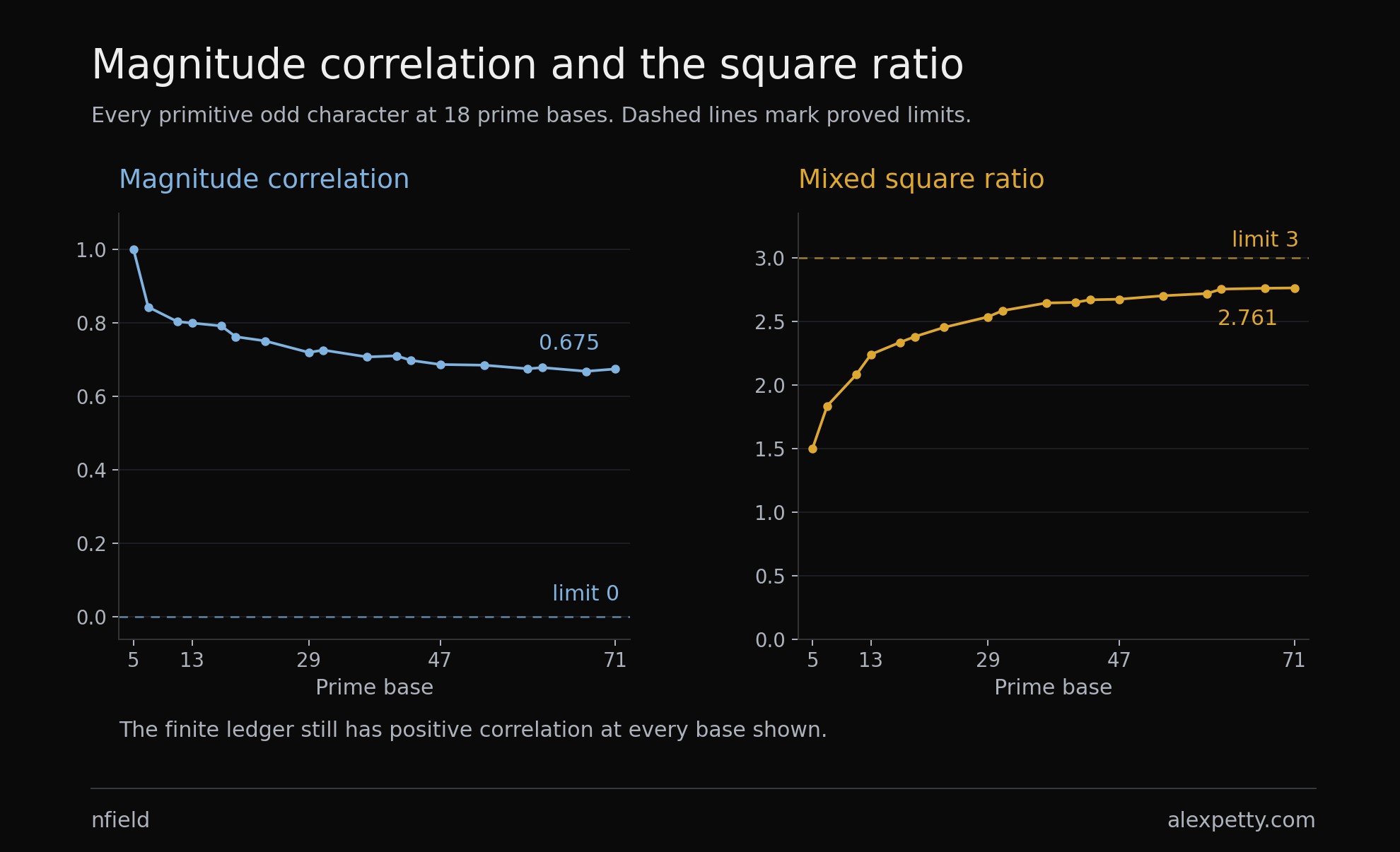
The Collision Spectrum ends with a question. Two magnitudes, both extracted from the digit function, keep rising and falling together. At base five the correspondence is exact. Their correlation is one. At base seven it is about $0.844$. By base seventy-one it is still about $0.675$.

Does that positive relation last as the base grows?

Its limit is zero.

The proof comes in three pieces. The first magnitude is a short character sum, read over a single block of digits. Adapting a recent and rather surprising theorem of Adam Harper, that character sums are typically a little smaller than a random walk of the same length would be, I show that most of these sums are small. The second magnitude is the size of a Dirichlet $L$-function at one, the kind of number that turns up in class number formulas and in the way primes spread through arithmetic progressions. I show that it has no runaway tail of large values, and that its spread never collapses to a single value. Together those three facts force the correlation to zero. They do it slowly. The bound shrinks like one over the fourth root of $\log\log b$, which is why the tables still show large positive values at base seventy-one.

Zero correlation is a weaker verdict than it sounds. Take any number between minus one and one, and square it. The square is completely determined by the number you started with. Know one and you know the other. Yet if you choose the number at random, the correlation between it and its square is zero. Correlation, the measure statisticians have used since Galton and Pearson, asks whether two quantities rise and fall together. It can miss a relation that is total.

But something survives. Square the magnitudes before comparing them, and a substantial relation persists. The average of their product approaches three times the product of their separate averages. The cubic law determines that three.

I want to show how both can be true.

Two walks on a circle of arrows

Make two walks from the arrows below. For the first, put arrows one through four end to end. For the second, use all twenty arrows, giving arrow $r$ a length of $r/25$.

Now measure the straight-line distance from each starting point to its endpoint. Forget how far the path travels. We want how far it gets.

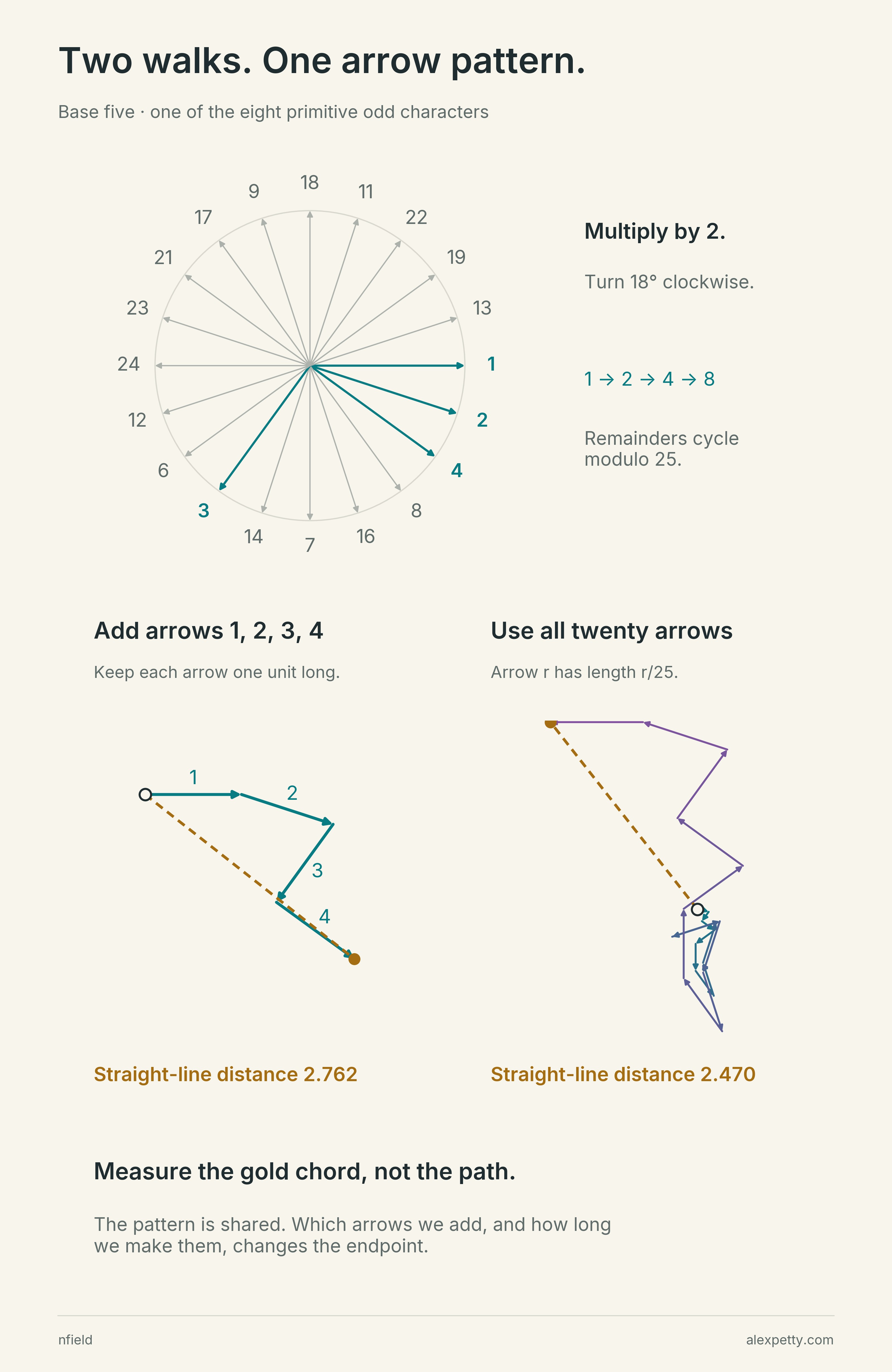
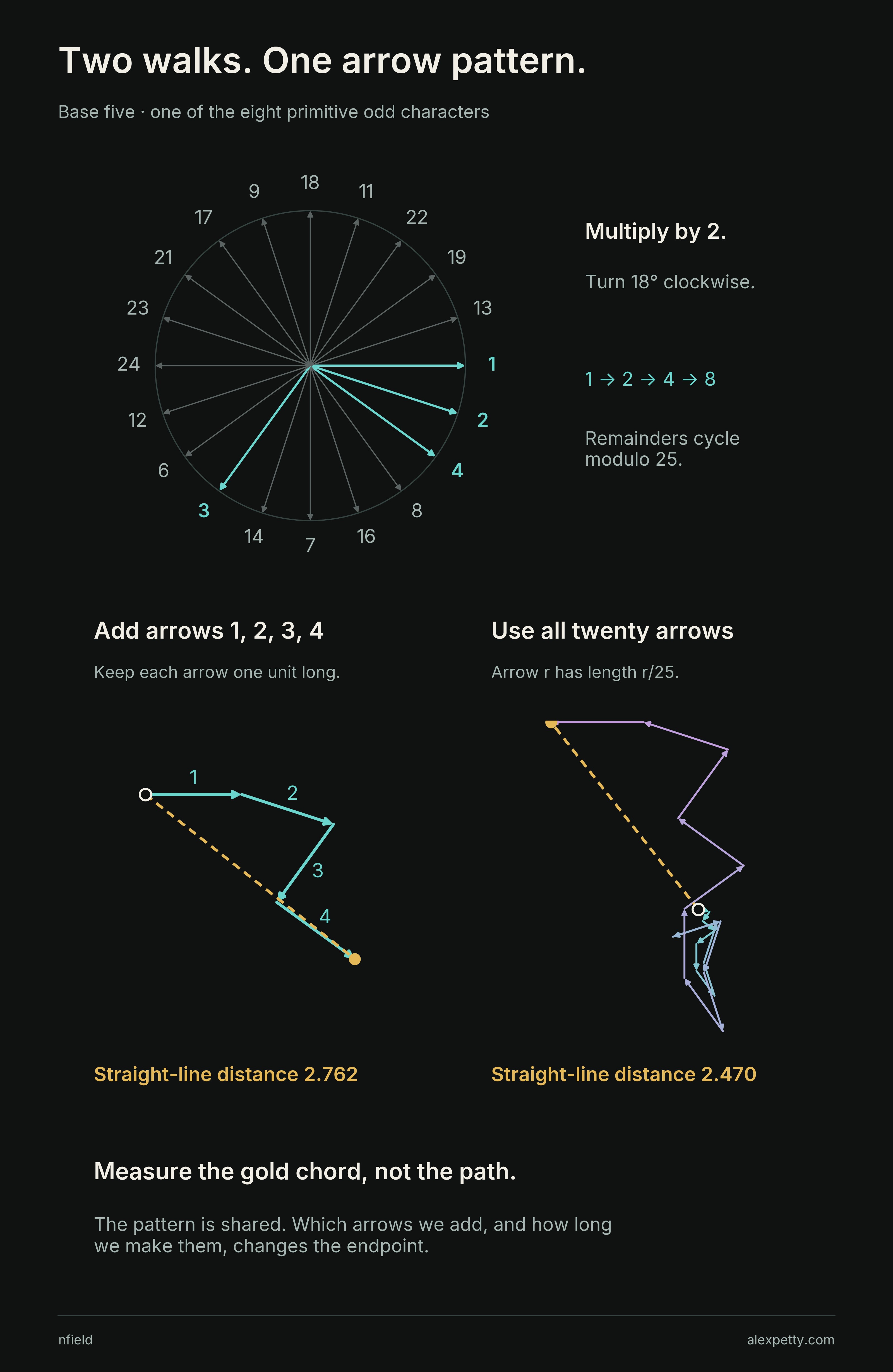
The arrows follow a multiplication rule. Multiplying their remainder labels adds their angles. In this base-five example, multiplying by two turns the arrow eighteen degrees clockwise. Multiples of five get zero weight, so they contribute no arrows. Such a pattern is called a character. Choose a different character and the arrows turn differently. Repeat the two walks and we have another pair of distances.

These distances come from the two factors in The Collision Spectrum. The short walk comes from the boundaries between digit bins. The weighted walk reads the whole remainder system. Its distance is also, after rescaling, the magnitude of an $L$-function value. Both come from the same arithmetic, but they read different parts of it.

For the character in the figure the short walk ends 2.762 from where it started and the weighted walk 2.470, which is exactly $2/\sqrt5$ of the first. At base five, the comparison uses eight characters, and all eight pairs share that ratio. A larger short-walk distance always comes with a larger weighted-walk distance, in the same ratio. Their ordinary correlation is one.

Eight pairs, sixty-four pairings

Stay at base five. Label the eight arrow patterns A through H. Each supplies a short distance and a weighted distance.

Square both distances and multiply them. Do that for the eight original pairs. Their average is exactly thirty.

Now let every short distance meet every weighted distance. A’s short walk can meet B’s weighted walk, or C’s, or its own. Eight choices on each side give sixty-four pairings. Their average squared product is exactly twenty.

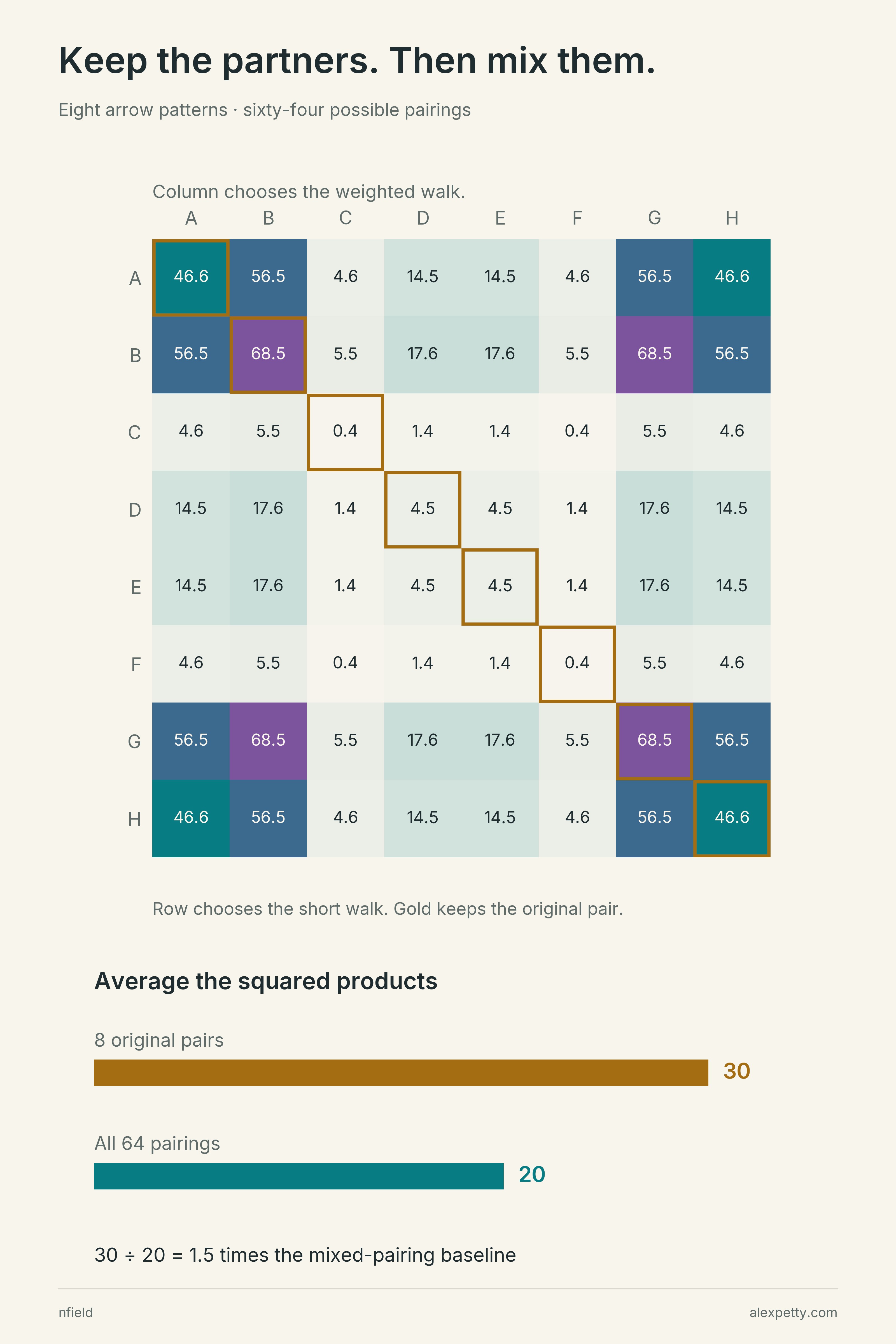
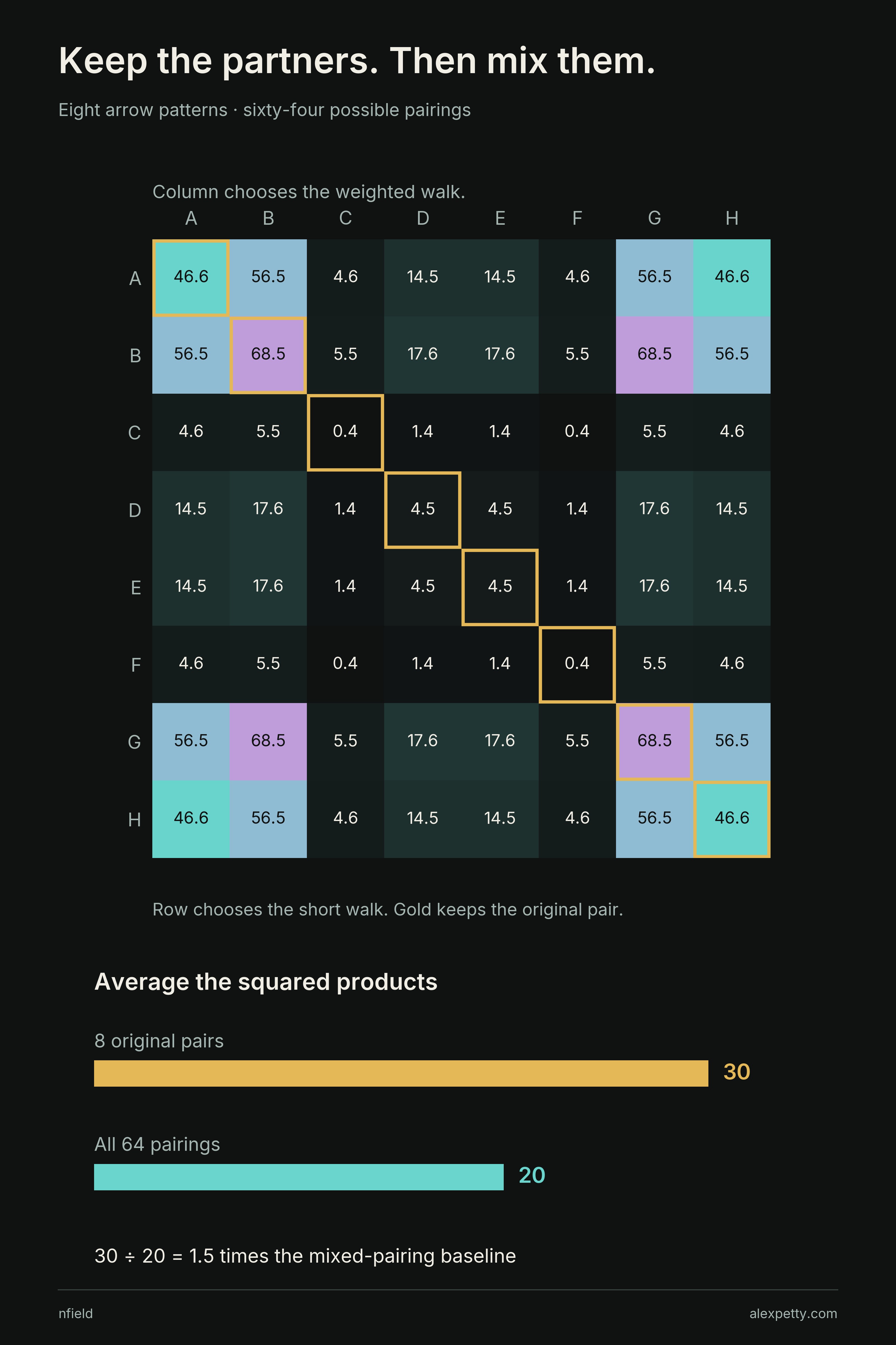
The gold diagonal keeps the original partners. The entire square mixes them. Keeping the partners gives $30/20=1.5$ times the mixed-pairing average.

There is no need to enumerate every new pair at a larger base. The all-pairings average is the product of the two separate averages. Call the ratio $R_b$,

$$R_b=\frac{\text{paired average}} {\text{mixed-pairing average}}.$$

At base seventy-one it is about $2.761$. Its limit is three. This is a ratio of averages rather than a correlation coefficient, so it is free to exceed one.

One large value among many

Squaring can change which part of a population controls the answer.

Take a hundred numbers. Ninety-nine are zero. The last is ten. Their average is $0.1$, but their average square is one.

Take ten thousand numbers. All but one are zero. The last is a hundred. The average falls to $0.01$. The average square is still one.

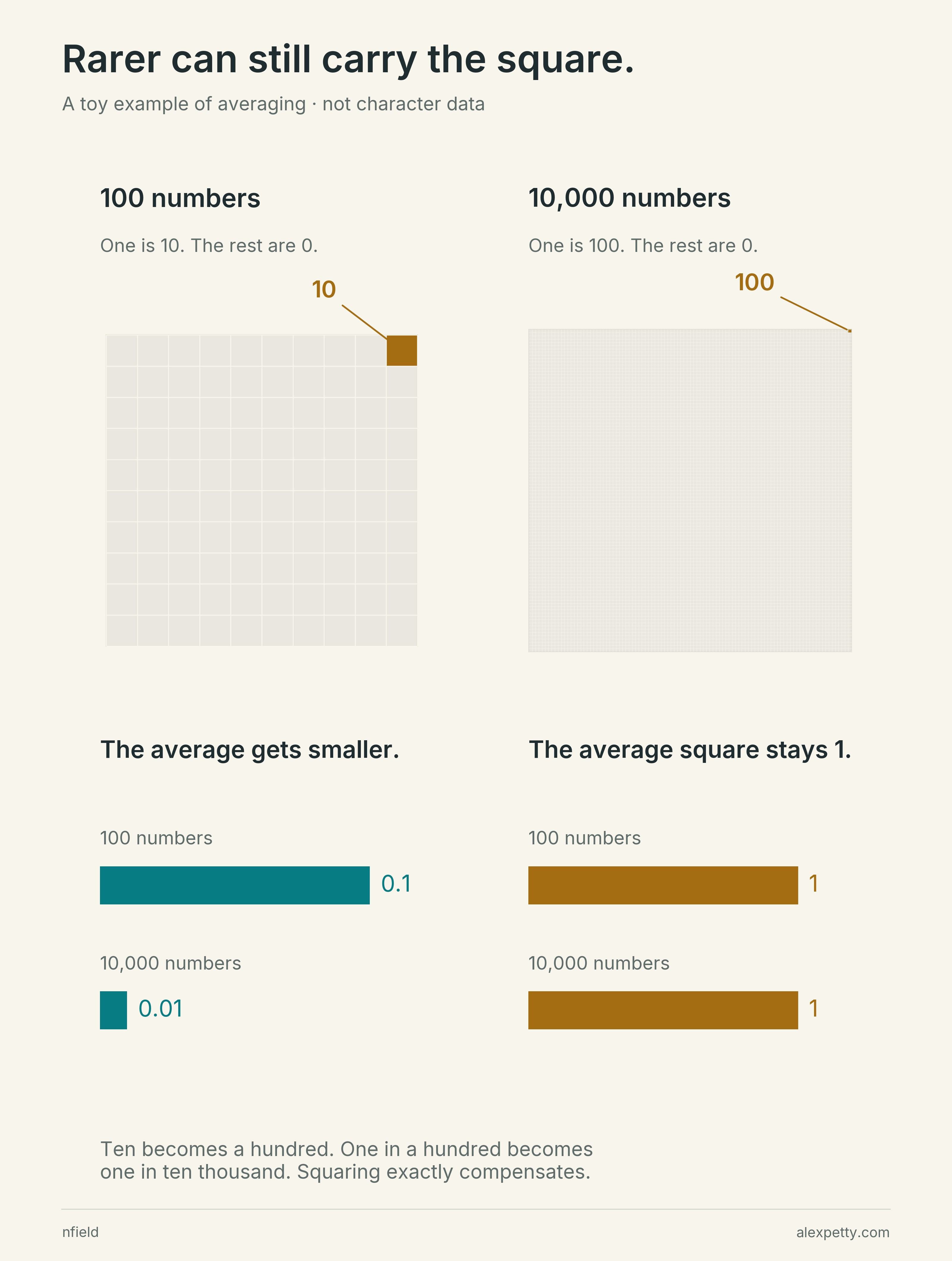
The exceptional value gets larger as it gets rarer. Squaring gives it enough weight to compensate exactly.

The short character sums do something of this kind. To compare different bases, divide each short distance by the square root of the base. The average square of these normalized distances is exactly one, at every prime base under consideration.

Their ordinary average nevertheless tends to zero.

This forces the square mass into a shrinking part of the family. Pick any fixed positive threshold. Eventually almost every normalized distance is below it, while almost all the square mass is above it.

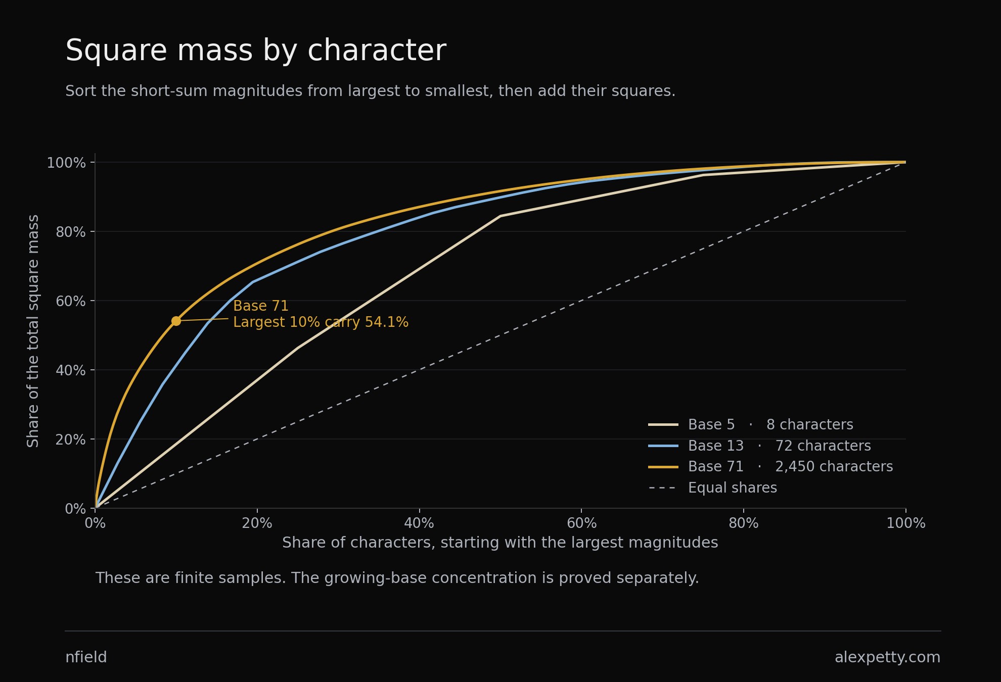
At base seventy-one we can see a finite version of that imbalance. The family contains 2,450 characters. Take the 245 largest short distances. They are a tenth of the family, yet they carry about $54.1$ percent of its square mass.

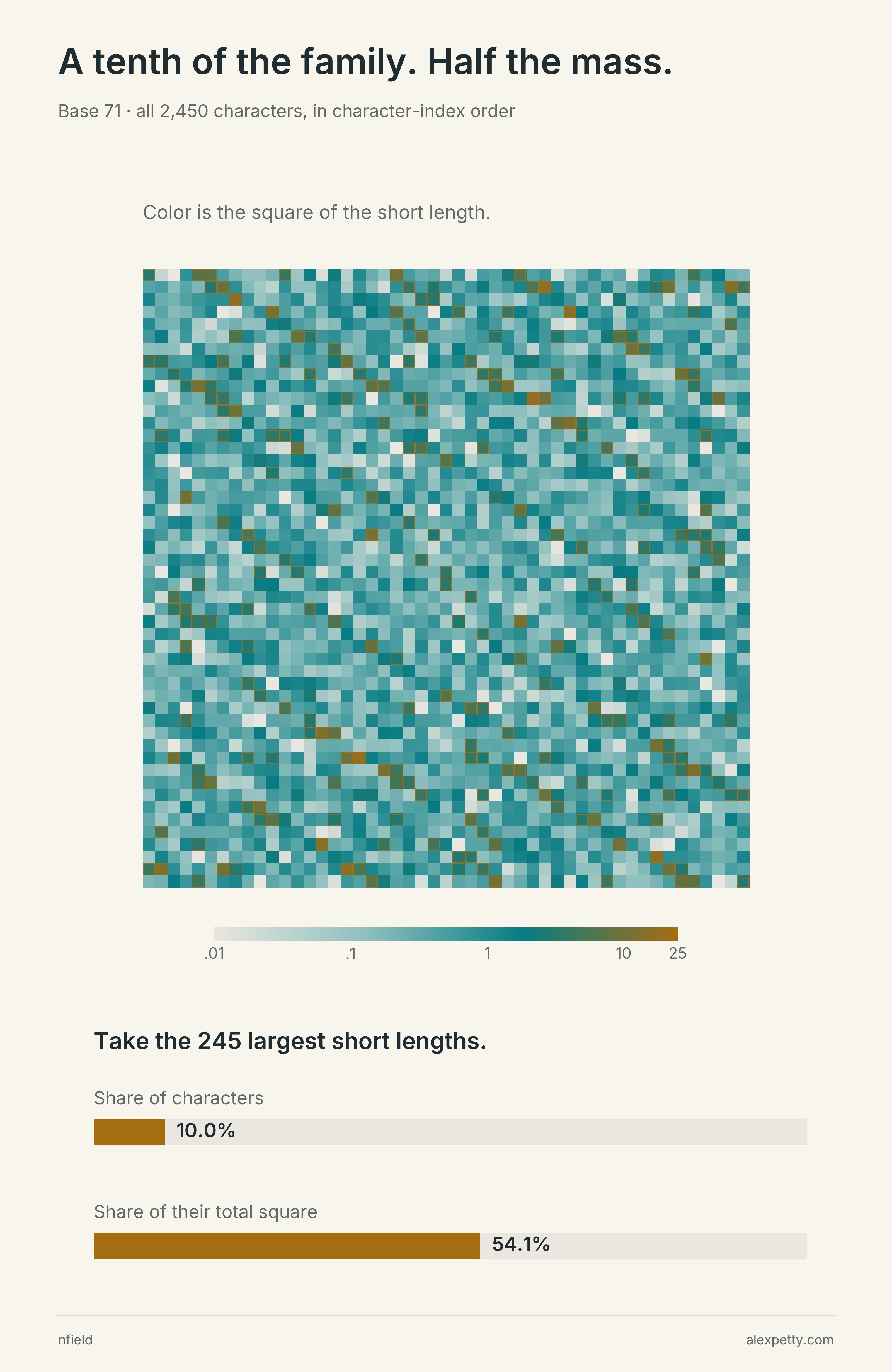
In the picture the outlined cells are scattered thinly through the field, each one a large value among ordinary neighbors. The bars underneath give the count, a tenth of the family holding more than half the mass. That is one base. The theorem says the imbalance keeps growing, until a vanishing fraction carries almost everything.

The proof has to catch the exceptions

Showing that most short distances are small is not enough. A few enormous values could still keep their average product with the weighted distances large.

The proof controls both sides. An estimate adapted from Adam Harper’s work on short character sums makes the average of the normalized short distances raised to the power $3/2$ tend to zero. That power lies between the ordinary average and the square average. It detects enough of the large values to close the gap.

On the other side, scale the weighted distances by $\pi/b$ so they too can be compared across bases. They have a bounded third moment, and their variance stays above a fixed positive amount. They neither grow an uncontrolled tail nor collapse to one common value.

Together these facts force the ordinary correlation to zero. The argument is unconditional. It does not assume the Riemann hypothesis or its generalization.

The squared comparison comes from a different result. Let $E_b$ be the collision energy, the sum of squares of the centered digit table. The exact identity is

$$R_b=\frac{3E_b}{(b-1)(b^2-1)}.$$

Digit Collisions and the Cubic Law proves that $E_b/b^3$ tends to one. The denominator grows like the same cube. That leaves the three. The Secondary Term of the Cubic Law gives its leading correction.

So the positive correlations in the tables fade, and still the arithmetic that paired the two walks leaves its mark. Keep those partners and square their distances. Even when the ordinary correlation has gone, breaking the pairs costs a factor of three.

The walks and the two comparisons, in notation

For a prime base $b\ge5$, work modulo $b^2$ with all $(b-1)^2/2$ primitive odd characters, including both members of every conjugate pair. A primitive character does not come from a smaller modulus. An odd character gives opposite arrows to opposite remainders. These are the restrictions supplied by the collision table’s centering and reflection.

The two walks are

$$T_b(\chi)=\sum_{k=1}^{b-1}\overline{\chi(k)},$$

$$B_{1,\overline\chi}=\frac1{b^2}\sum_{a=1}^{b^2-1}a\overline{\chi(a)}.$$

Character values at multiples of $b$ are zero. The diagonal factor in the collision spectrum is $-2\overline{\chi(b+1)}T_b(\chi)$. Its magnitude is therefore twice the short-walk distance. The weighted walk satisfies the classical special-value identity

$$|B_{1,\overline\chi}|=\frac b\pi|L(1,\chi)|.$$

The normalized variables used in the atlas are $X=|T_b|/\sqrt b$ and $Y=\pi|B_{1,\overline\chi}|/b=|L(1,\chi)|$. Positive rescaling of either variable changes neither the ordinary correlation nor the squared-product ratio. Thus the raw distances in the eight-by-eight example give the same $R_5$ as the normalized variables.

With averages over the character family,

$$\mathbb E X^2=1,$$

$$\mathbb E Y^2=\nu_b=\frac{\pi^2}{6}\left(1-\frac1{b^2}\right),$$

$$r_b=\frac{\mathbb E(XY)-\mathbb E X\,\mathbb E Y} {\sqrt{\operatorname{Var}(X)\operatorname{Var}(Y)}},$$

$$R_b=\frac{\mathbb E(X^2Y^2)}{\mathbb E X^2\,\mathbb E Y^2}.$$

At base five, $|B_{1,\overline\chi}|=2|T_5(\chi)|/\sqrt5$ for every character in the family. The separate raw square averages are five and four. Their product is twenty, and the paired square-product average is thirty. Letters A through H in the figure are character indices $1,3,7,9,11,13,17,19$ for the generator two modulo twenty-five.

From fractional moments to decorrelation

Harper’s stated theorem uses a prime modulus. The paper checks its transfer to this prime-square family, including the product-size and unit conditions required by character orthogonality. It does not simply substitute $b^2$ into a prime-modulus theorem.

Writing $H_b=\mathbb E X^{3/2}$, the transferred estimate gives

$$H_b\ll(\log\log b)^{-3/8}.$$

Hölder’s inequality gives $\mathbb E X\le H_b^{2/3}$ and

$$\mathbb E(XY)\le H_b^{2/3}(\mathbb E Y^3)^{1/3}.$$

The third moment of $Y$ is uniformly bounded. Since $\mathbb E X^2=1$, the variance of $X$ tends to one. The exact identities $\mathbb E\chi(2)=0$ and $\mathbb E[Y^2\chi(2)]=\nu_b/2$ yield $\operatorname{Var}(Y)\ge\nu_b/16$. These bounds keep the correlation denominator away from zero and give

$$|r_b|=O\!\left((\log\log b)^{-1/4}\right).$$

The slow double-logarithmic bound is compatible with positive correlations throughout the finite calculations. It is a proof of the limit, not a useful numerical prediction at these bases.

For the square ratio, the secondary energy term gives

$$\begin{aligned} R_b={}&3-\frac3{\pi^2}\frac{(\log b)^2}{b}\\ &+O\!\left(\frac{\log^2(2b)}{b\log\log(3b)}\right). \end{aligned}$$

In particular, $\operatorname{Cov}(X^2,Y^2)\to\pi^2/3$. Neither this covariance nor $R_b$ is the Pearson correlation of the squared variables.

Inspect the character families

Every character contributes one point with horizontal coordinate $X$ and vertical coordinate $Y$. Conjugate characters have identical magnitudes, so their points coincide. The atlas counts both.

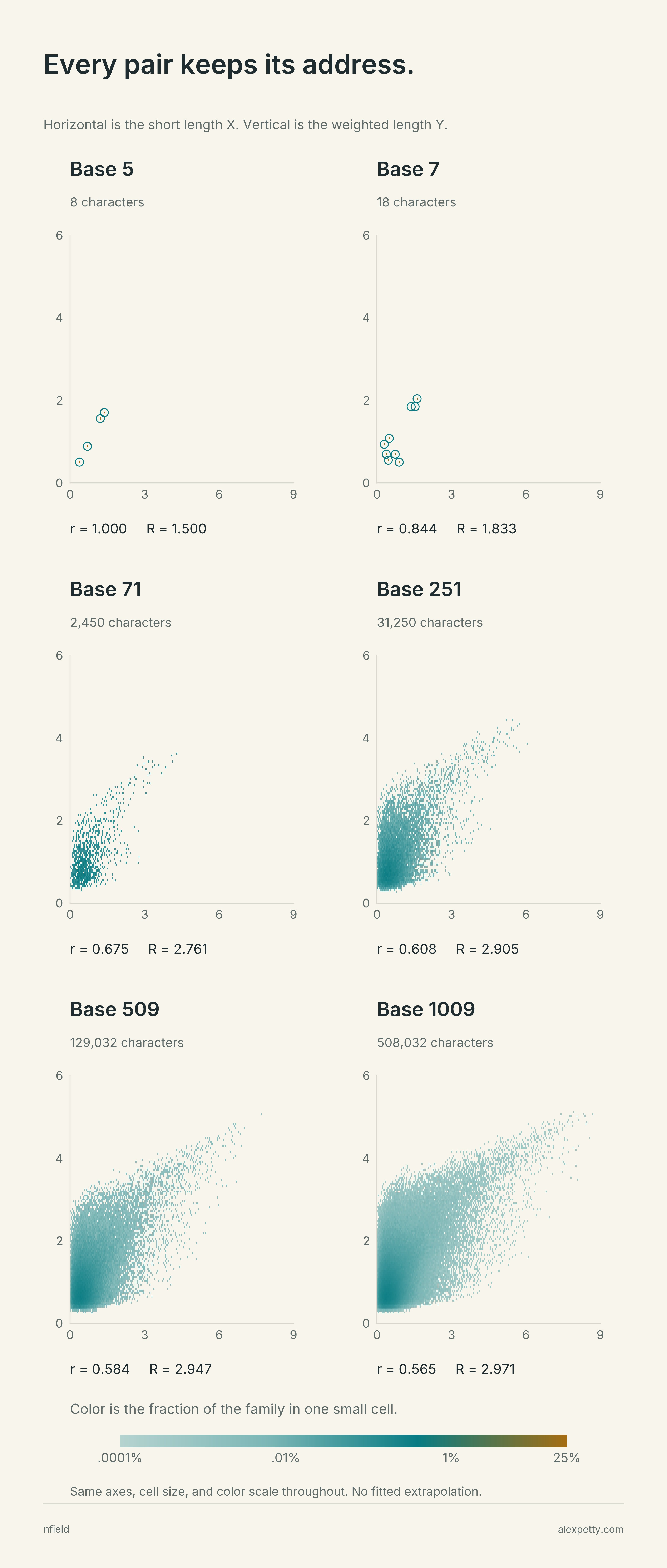
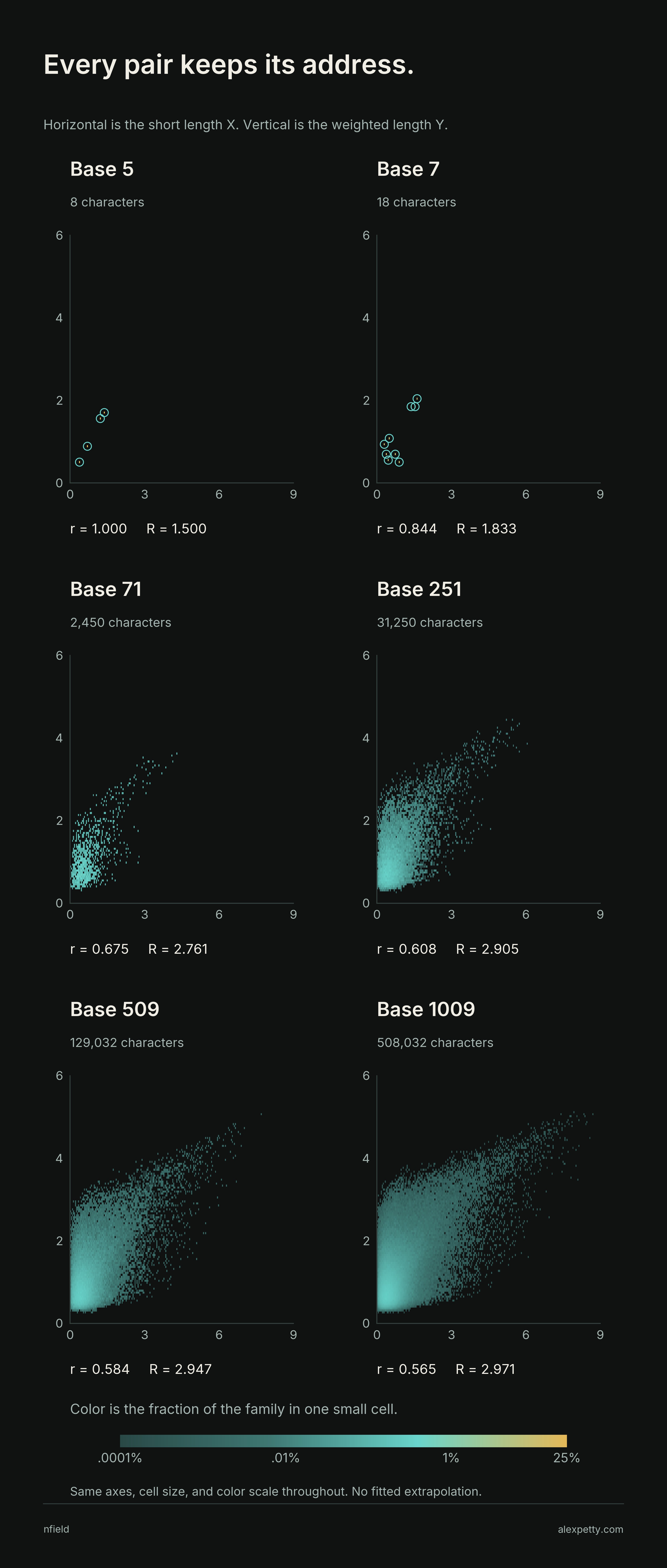
Each small cell has the same dimensions in all six panels. Its color is the fraction of the family falling inside it, on one fixed logarithmic scale. Empty cells remain blank. Outlines make the few occupied cells at bases five and seven visible at reading size. They add no observations.

Base	Characters	Correlation r	Square ratio R
5	8	1.0000	1.5000
7	18	0.8440	1.8333
13	72	0.8004	2.2381
29	392	0.7203	2.5327
71	2,450	0.6753	2.7608
251	31,250	0.6082	2.9047
509	129,032	0.5841	2.9468
1,009	508,032	0.5646	2.9712

The paper’s ledger contains all eighteen prime bases from five through seventy-one, totaling 14,372 characters. I also ran the bases 101, 251, 509 and 1,009. Across both sets, the computation covers 687,686 characters. The atlas shows six of these families, not every base in the ledger.

Character sums are recomputed by a finite Fourier transform and checked against direct summation. The original ledger is also checked against the native C implementation. The square ratios agree with the exact finite collision energies. These checks verify the examples, not the asymptotic theorems. The finite correlation is not monotone at every prime.

The finite comparison plots

The eighteen-base ledger can also be read as two curves. These plots keep the ordinary correlation, the square ratio and the concentration of square mass together for comparison.

The paper and its sources

The full statements, proofs and finite verifiers are in Magnitude Decorrelation in the Collision Spectrum. The fractional-moment method comes from Adam Harper, The typical size of character and zeta sums is $o(\sqrt{x})$. The manuscript separates that method, its prime-square transfer and the exact collision-energy identities.

The spectral factorization is introduced in The Collision Spectrum, the cubic energy law in Digit Collisions and the Cubic Law, and its secondary term in The Secondary Term of the Cubic Law.