The Analytic Collision Transform

The collision coefficient at base five is an average of twenty signed fractions from long division. For the character that turns eighteen degrees at each power of two, it comes to about $0.441164-0.520524i$. Its size carries $L(1,\chi)$, as The Collision Spectrum and the L-Function Landscape showed, and I wanted to know whether the rest of the $L$-function could be reached from the same table. It can, with classical tools. Place the periodic zeta function on the diagonal of equal digit pairs and take the character transform, and the result is a fixed multiple of $L(s,\overline\chi)$ throughout the critical strip, with the collision coefficient sitting at $s=0$.

The fixed multiple is the same five-step sum over the diagonal of equal digit pairs, and it doesn’t change as $s$ moves. The rest of the factor is a gamma function and a sine, which never vanish for $0<\operatorname{Re}s<1$. So whenever the digit sum is nonzero, the transform has exactly the zeros of $L(s,\overline\chi)$ there, with the same multiplicities, which follows at once from the factorization and says nothing new about where those zeros are. The new part is the factorization itself, with the finite digit sum carried through unchanged and the collision coefficient recovered at the left edge, phase and all, times $i\pi$.

An eighteen-degree turn

A character modulo $25$ gives each residue a complex weight, and multiplying residues multiplies their weights. Successive powers of $2$ visit all twenty residues not divisible by five, so a character is set by how far it turns at each visit. Take the one that turns eighteen degrees, $\chi(2)=e^{\pi i/10}$, and give the multiples of five weight zero.

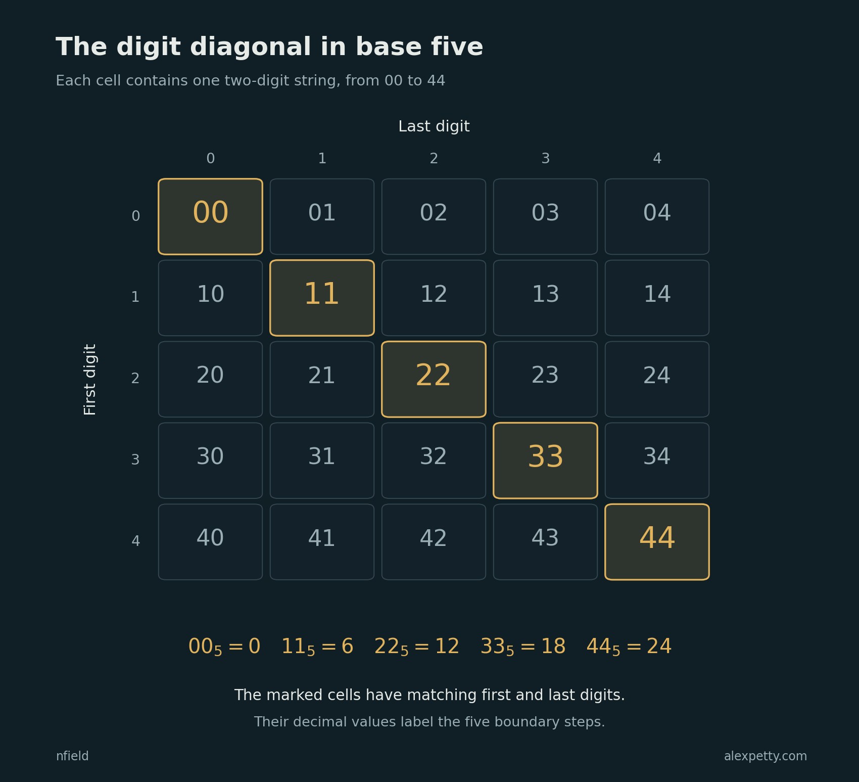
The base-five words with equal digits, $00$, $11$, $22$, $33$ and $44$, are the integers $0$, $6$, $12$, $18$ and $24$. Step each forward by one, wrapping $24$ around to $0$, and record how much the character’s weight changes across each step. Adding the five changes gives

$$\begin{aligned} G&=\{0,6,12,18,24\},\\ D(\chi)&=\sum_{n\in G}[\chi(n+1)-\chi(n)]. \end{aligned}$$

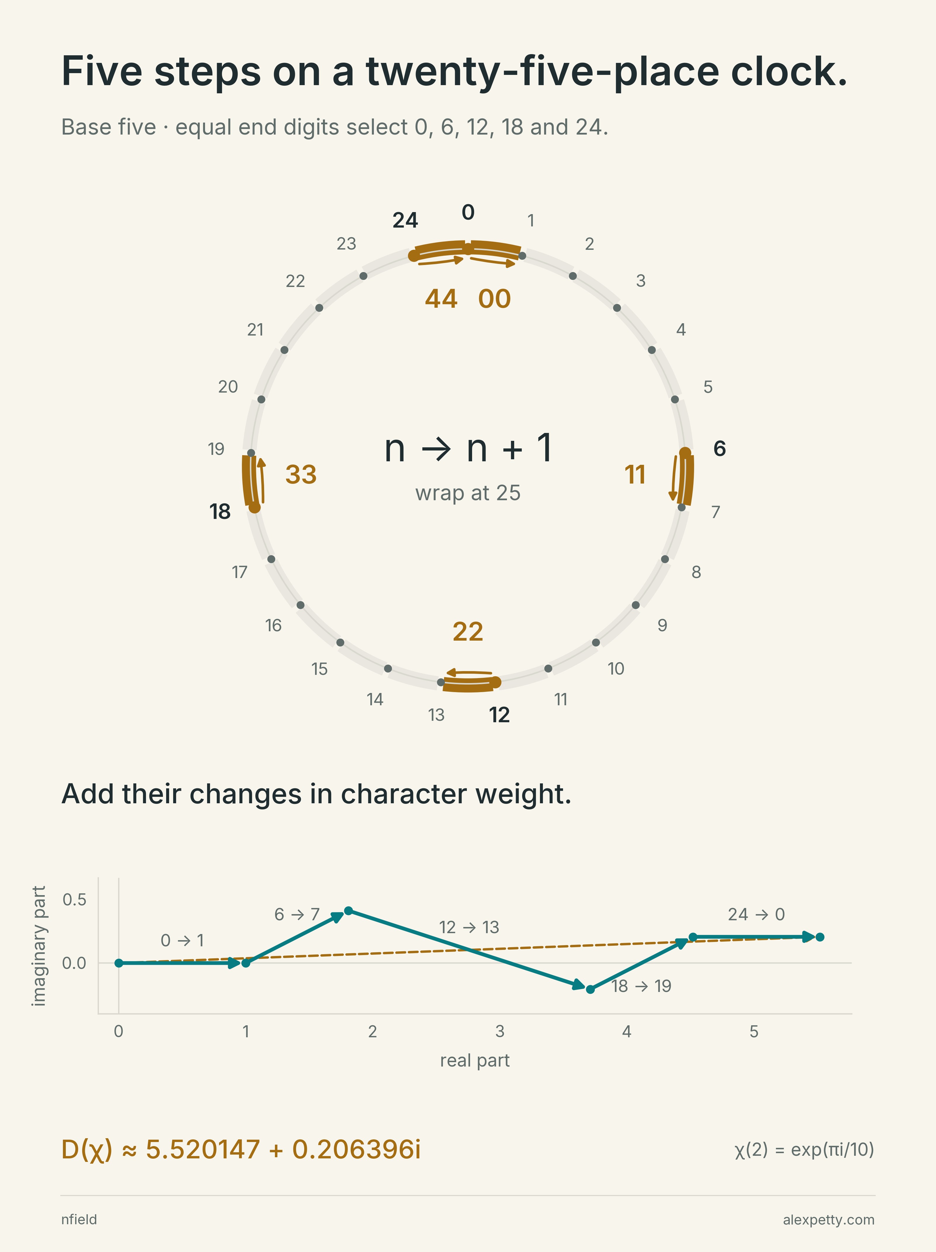
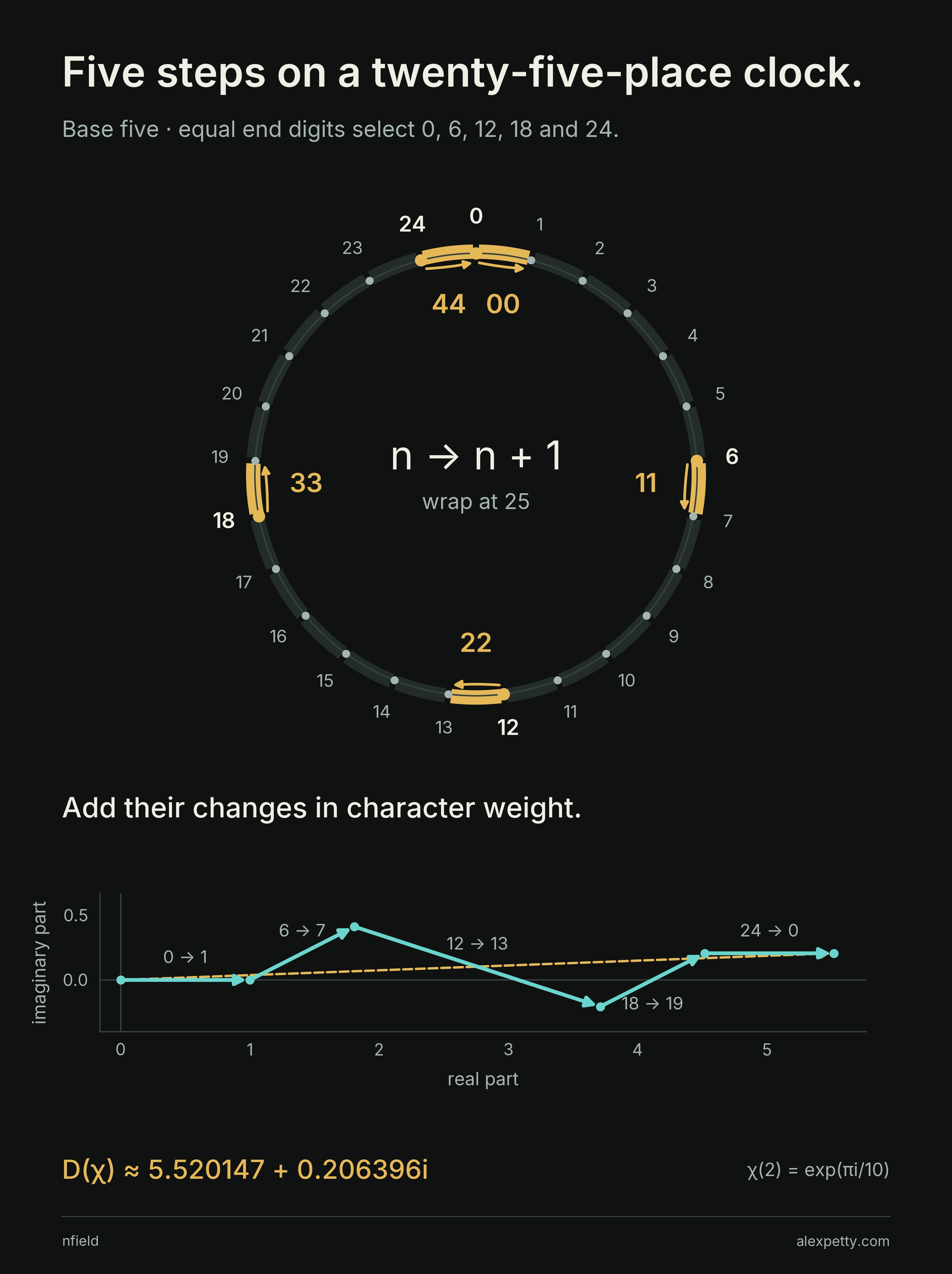
On the clock the five steps are the short gold arcs at $00$, $11$, $22$, $33$ and $44$. Below, their weight changes are drawn head to tail. The first arrow, from $0$ to $1$, is exactly one unit along the real axis, and so is the last, from $24$ back to $0$, because $\chi(24)=-1$ and $\chi(0)=0$. The three middle steps zigzag up and down between them, and the five arrows land at

$$D(\chi)\approx5.520147+0.206396i.$$

Nothing analytic has happened yet. Once the base, lag and character are chosen, this number is finished.

The character convention and larger digit tables

Here $D$ uses $\chi$ directly. It is the conjugate of the diagonal factor $D_\chi$ in The Collision Spectrum and the L-Function Landscape. The collision coefficient is unchanged by this notation choice.

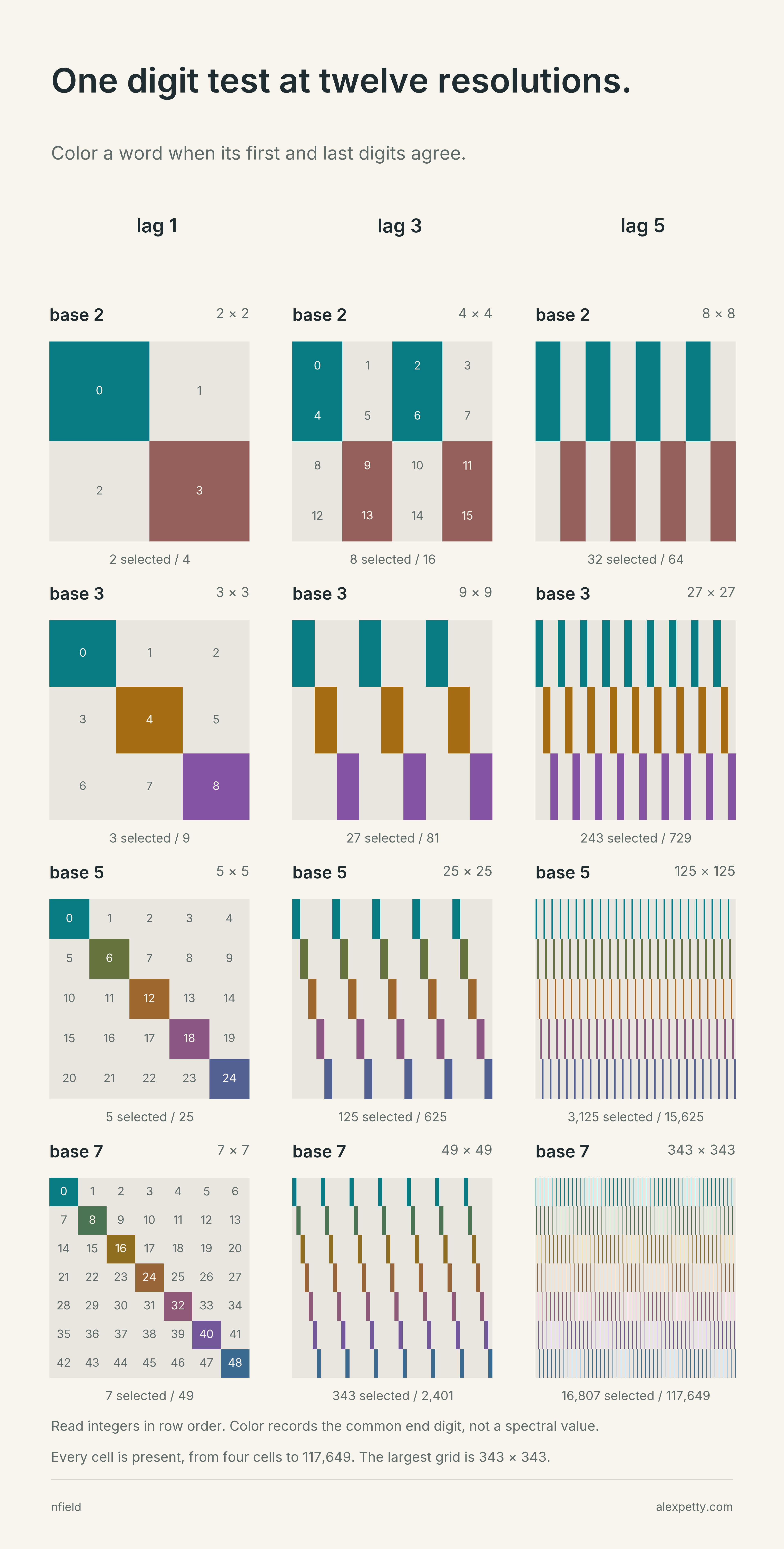
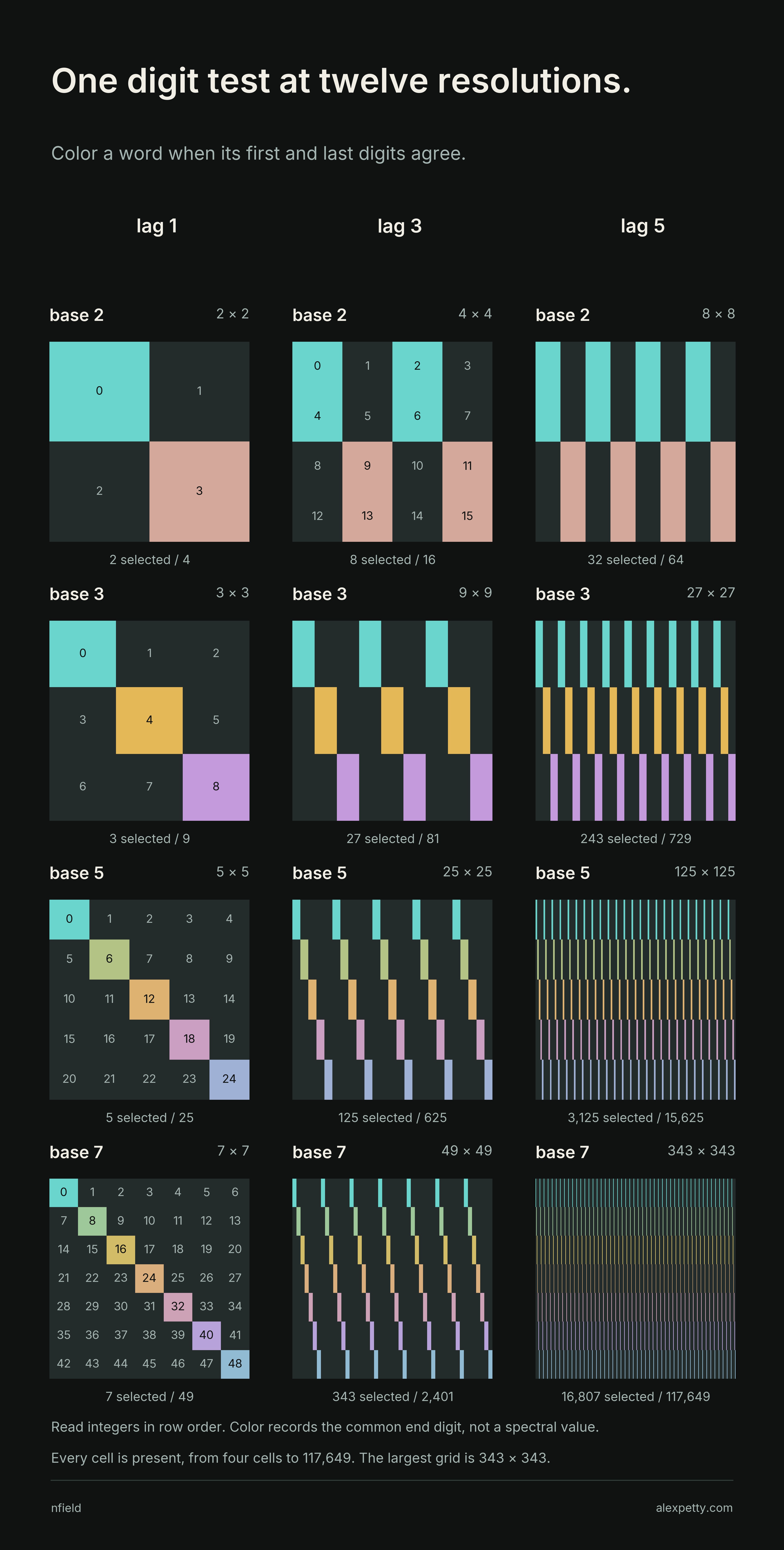
At lag $\ell$, the words have $\ell+1$ digits, including leading zeros. Their first and last digits must agree. There are $b^\ell$ such words among $m=b^{\ell+1}$ possibilities. Write their integer labels as $G_\ell$ and use

$$D_\ell(\chi)=\sum_{n\in G_\ell}[\chi(n+1)-\chi(n)].$$

The gallery places all the integers in row order. At lag one this gives the familiar diagonal. With more intervening digits, the selected cells spread into bands. The colors identify the common end digit.

Arrows that reach farther

The analytic family needs a kernel, and the classical one is the periodic zeta function. Put a turning arrow at each positive integer $j$, pointing $jx$ full turns around, give it length $1/j^{1-s}$ for real $s$, and add the arrows head to tail,

$$K(x;s)=\sum_{j=1}^{\infty}\frac{e^{2\pi i jx}}{j^{1-s}}.$$

At $s=0$ the lengths are $1,1/2,1/3,\ldots$, and at $s=1/2$ they are $1,1/\sqrt2,1/\sqrt3,\ldots$.

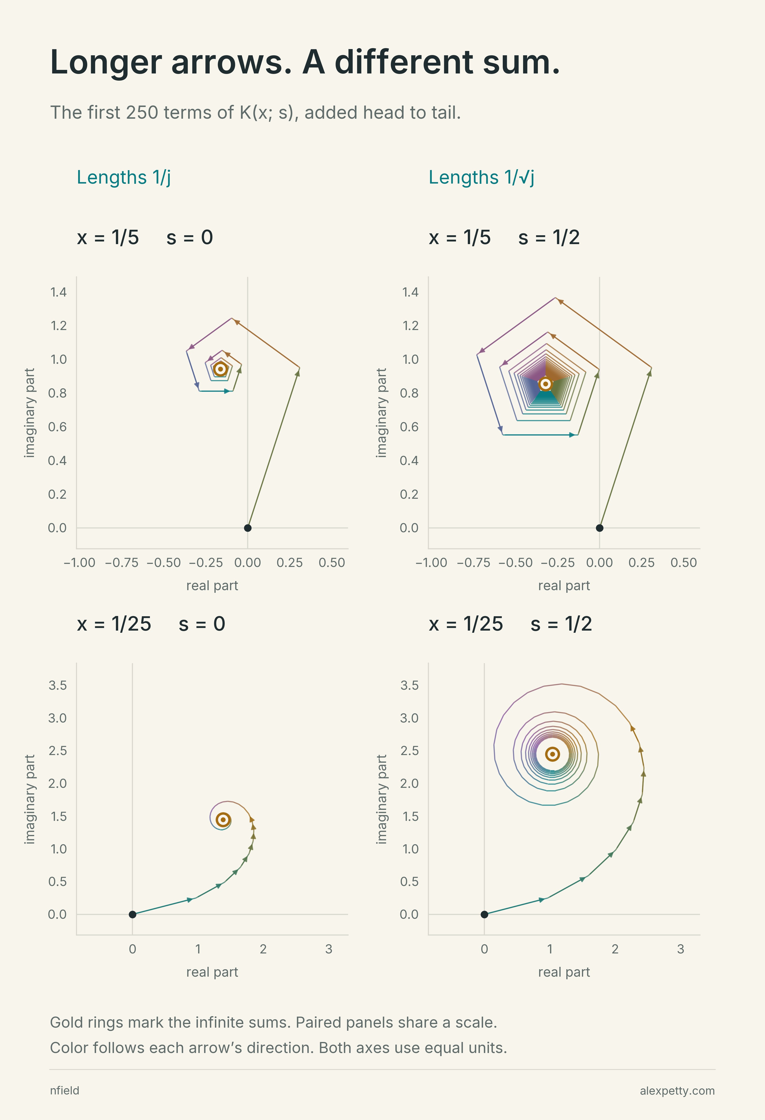
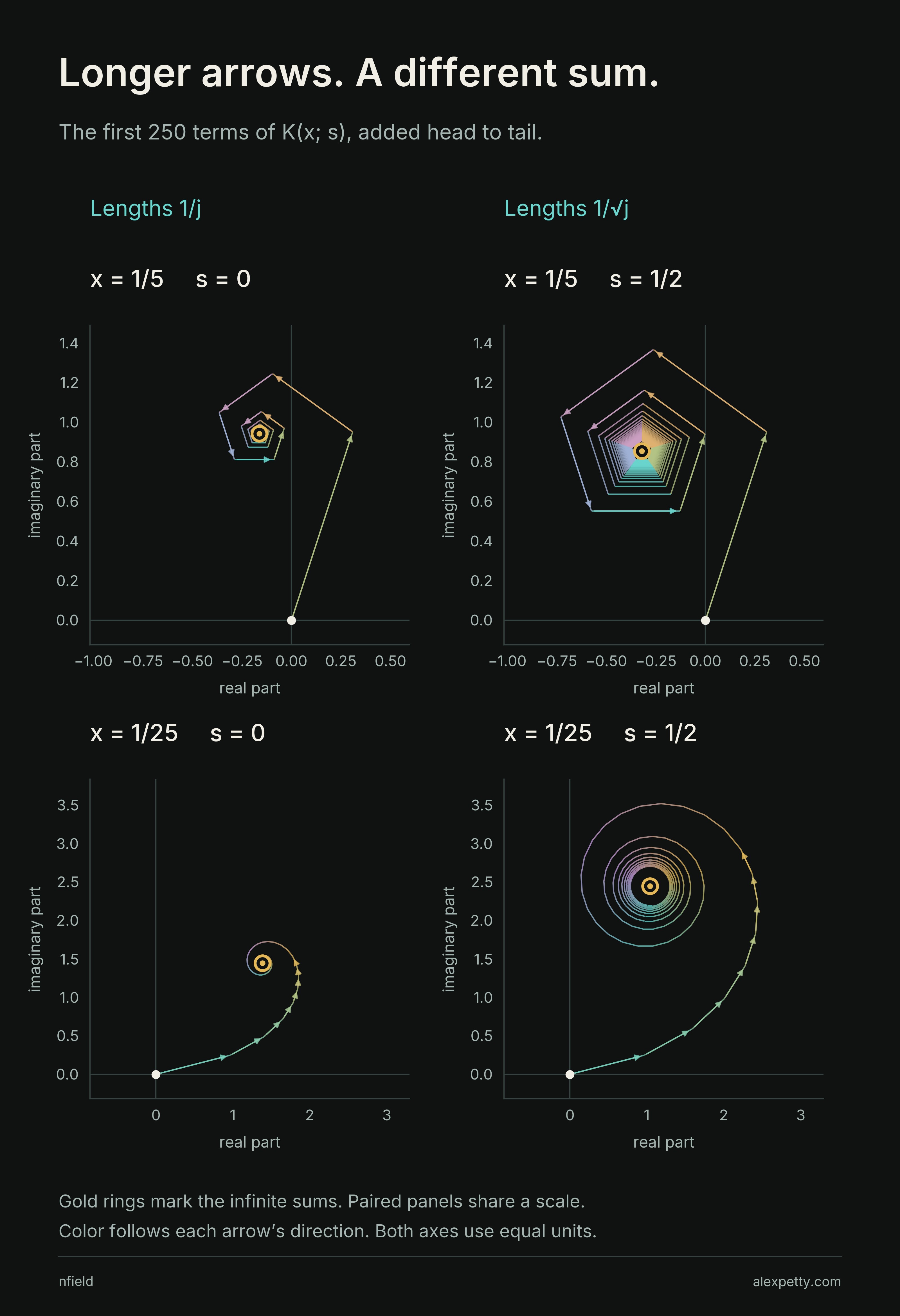
At $x=1/5$ each arrow turns a fifth of a circle from the last, so the path winds in pentagons. With lengths $1/j$ the pentagons shrink quickly and close on the gold ring within a few laps. With lengths $1/\sqrt j$ they stay wide and wind many more times before settling, around a different sum. At $x=1/25$ the turns are smaller and the path curls into a spiral. For $0<x<1$ the series converges whenever $\operatorname{Re}s<1$, analytic continuation supplies its values beyond that, and a complex $s=\sigma+it$ adds a further turn of $t\log j$ radians to the $j$th arrow.

At $s=0$ the kernel has a very simple imaginary part,

$$\frac{\operatorname{Im}K(x;0)}{\pi}=\frac12-x,$$

a straight line, and that line is the Bernoulli factor of the finite collision calculation, already sitting inside the kernel.

Cancel the shared endpoint

Now put the kernel on the five steps. Multiply each step by an allowed residue $a$, reduce both ends modulo $25$, divide by $25$, and take the kernel at the finishing end minus the kernel at the starting end. One pair of steps needs care. With $a=2$ the first step becomes $0\to2$ and the last becomes $23\to0$, so both reach the kernel at zero, where its series diverges.

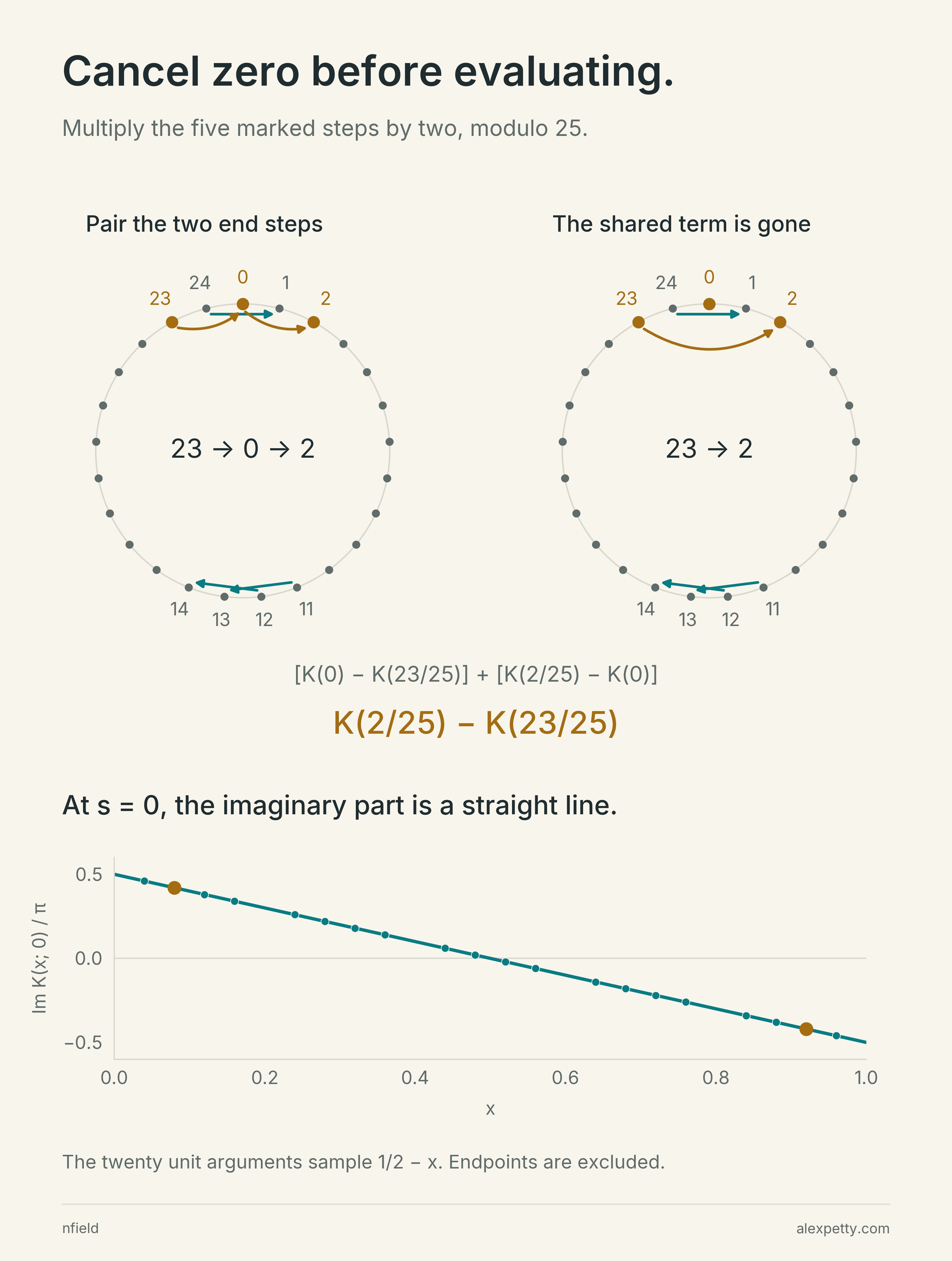
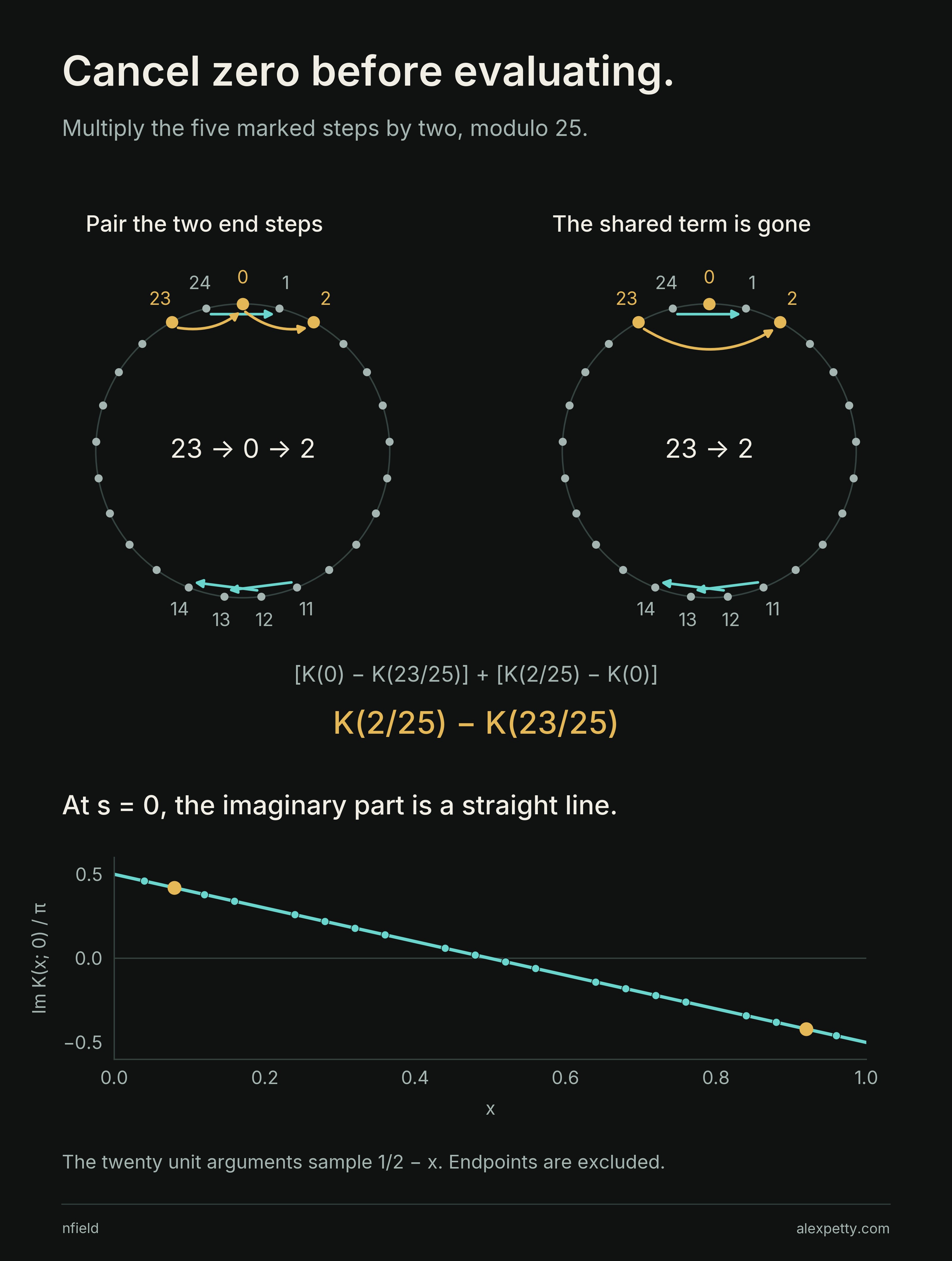
The left clock shows the two end steps meeting at $0$, and the right clock shows them joined into a single step from $23$ to $2$. Written out,

$$[K(0)-K(23/25)]+[K(2/25)-K(0)]=K(2/25)-K(23/25),$$

so the value at zero never has to be computed. The line at the bottom is the imaginary part of the kernel at $s=0$, the line $1/2-x$, with the twenty allowed arguments as dots and the two gold ones at $2/25$ and $23/25$.

Doing this for all twenty allowed values of $a$, subtracting the mean within each final-digit family as in the centered collision table, and averaging against the conjugate character weights gives the transform $\mathcal A_\chi(s)$.

The complete definition

Let $\{y\}$ mean the fractional part of $y$. At modulus $m=b^{\ell+1}$, the uncentered quantity is

$$\begin{aligned} A(a;s)=\sum_{n\in G_\ell}\bigl[&K(\{(n+1)a/m\};s)\\ &-K(\{na/m\};s)\bigr]. \end{aligned}$$

Combine the terms from $n=0$ and $n=m-1$ first. Their contribution is $K(a/m;s)-K(1-a/m;s)$, so every argument actually evaluated lies strictly between zero and one.

Write $U_m$ for the residues coprime to $m$. For a prime base, each final-digit family contains $b^\ell$ of them. Subtract its mean,

$$\begin{aligned} A^\circ(a;s)&=A(a;s)\\ &\quad-\frac1{b^\ell}\sum_{\substack{u\in U_m\\u\equiv a\pmod b}}A(u;s). \end{aligned}$$

Then take the character coefficient,

$$\mathcal A_\chi(s)=\frac1{\varphi(m)} \sum_{a\in U_m}A^\circ(a;s)\overline{\chi(a)}.$$

Here $\varphi(m)$ counts the allowed residues. It is $20$ at modulus $25$.

Five steps survive the transform

Inside the critical strip, $0<\operatorname{Re}s<1$, the result factors exactly,

$$\mathcal A_\chi(s)=C_m(s)D_\ell(\chi)L(s,\overline\chi),$$

for every prime base and every primitive odd character. Primitive means the character needs the full modulus, and odd means reflection changes its sign. The eighteen-degree character is both.

The proof follows those two properties through the sum. Multiplying by a residue coprime to $m$ only rearranges the kernel arguments and brings out a character value. For a residue sharing a factor with $m$, primitivity makes the weights cancel. Oddness pairs each kernel term with its reflection and leaves a sine. The digit geometry comes through untouched as the same five-step sum $D$ the calculation started with.

The common factor and the proof

The factor independent of the character is

$$C_m(s)=\frac{2i\sin(\pi s/2)\Gamma(s)}{\varphi(m)} \left(\frac{m}{2\pi}\right)^s.$$

For a primitive character, its sum over every fiber of reduction to a smaller prime-power modulus is zero. That removes the family-centering term and all nonunit kernel models. On the remaining unit models, the periodic-zeta connection formula expresses the kernel in terms of two Hurwitz zeta functions. The finite character-weighted Hurwitz sum is $m^sL(s,\overline\chi)$. Reflection and oddness supply $2i\sin(\pi s/2)$.

The Analytic Collision Transform gives the fiber-cancellation argument, endpoint accounting, factorization and both boundary proofs.

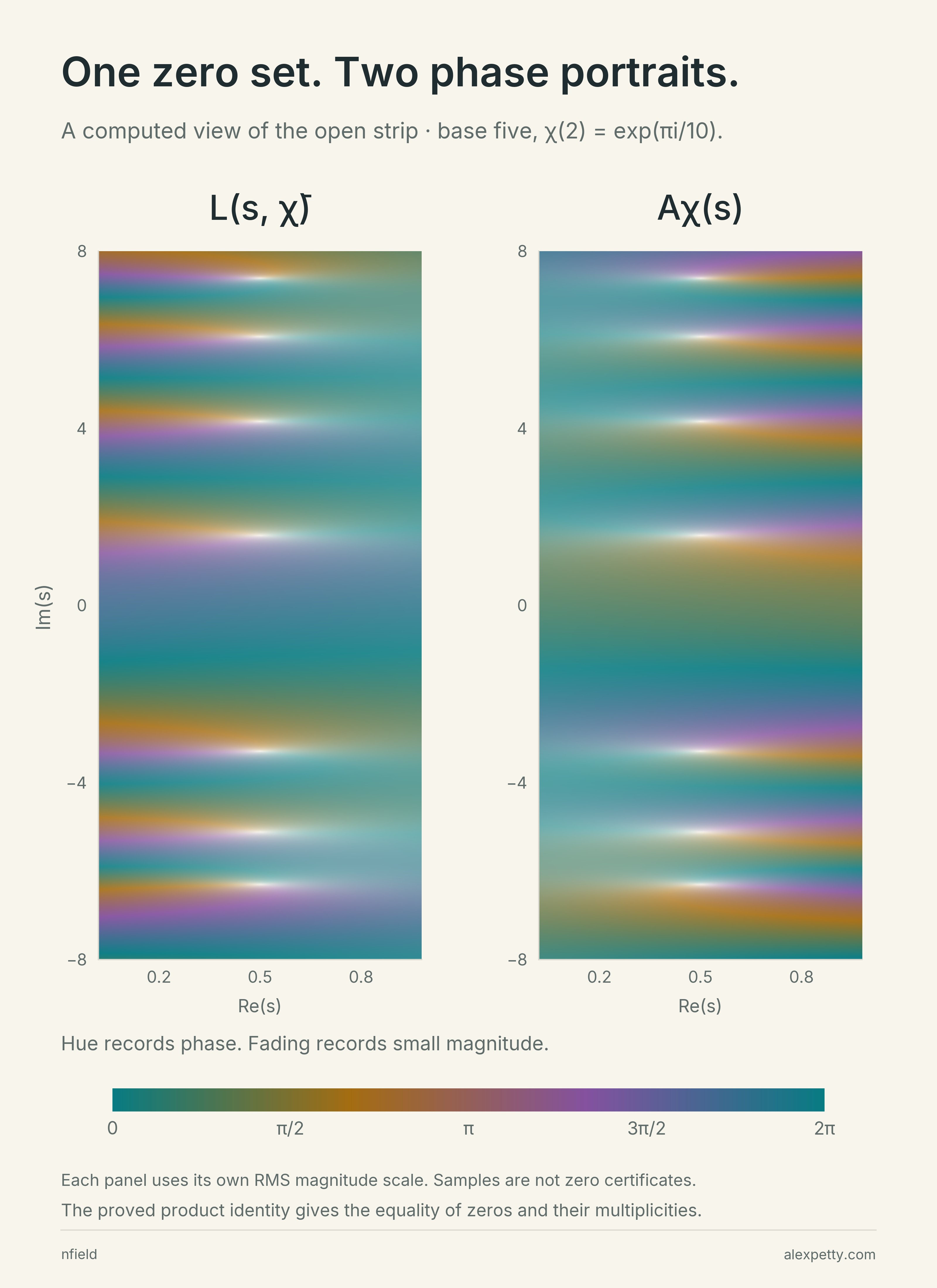
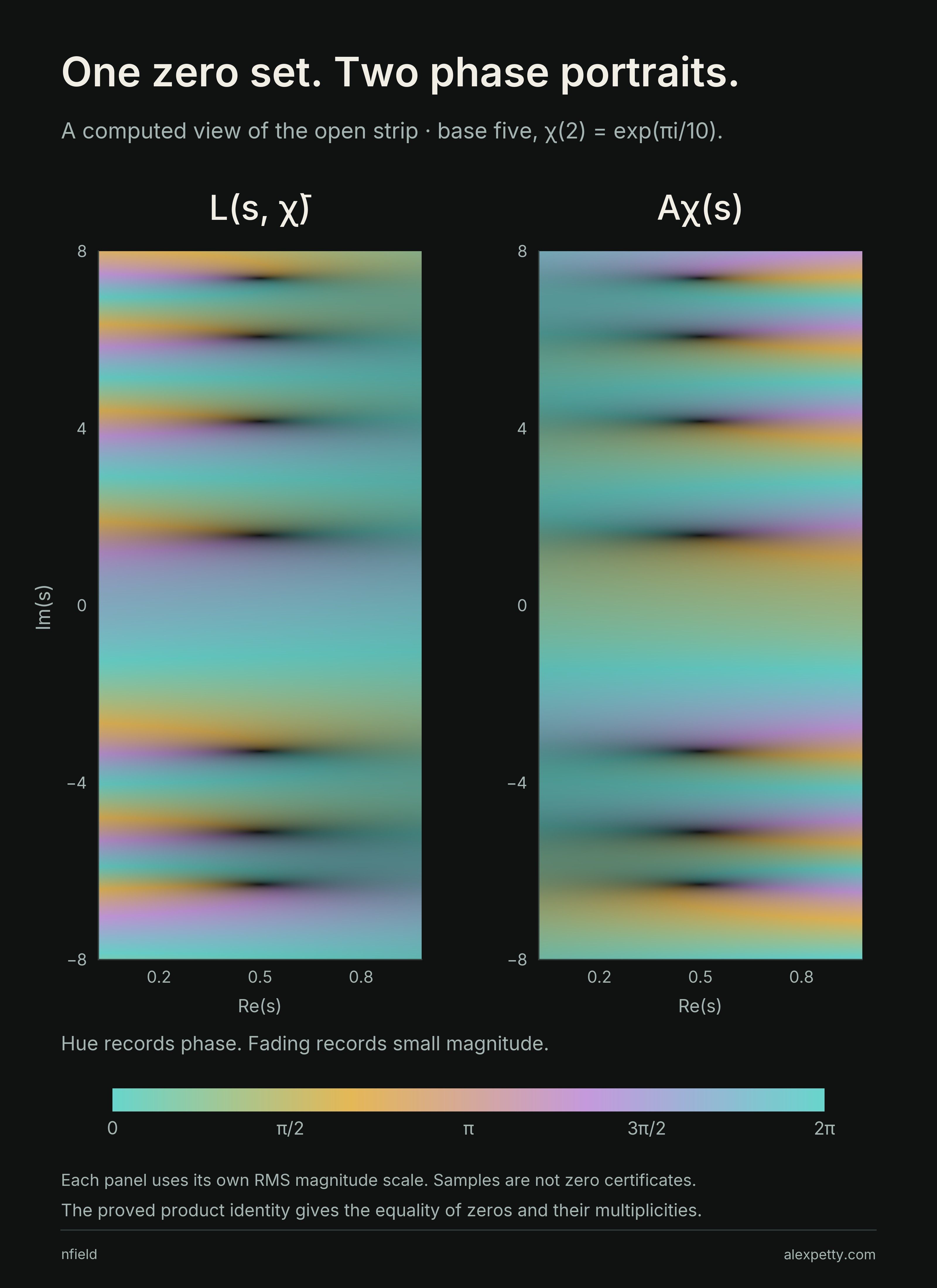
The two panels color the same rectangle of the critical strip by phase, $L(s,\overline\chi)$ on the left and the transform on the right. The colors differ, because multiplying by $C_m(s)D(\chi)$ shifts every phase and size, but the bright pinch points, where all the colors meet, line up row for row in the two panels. The theorem is what makes that exact. The common factor never vanishes in the critical strip and $D(\chi)$ is nonzero, so the two functions have the same zeros with the same multiplicities. The picture only illustrates it. A character whose five-step sum vanished would have its whole component vanish instead. At modulus $25$ none does, since all eight primitive odd characters have nonzero diagonal sums.

All eight primitive odd components

At modulus $25$, write $\chi_j(2)=e^{2\pi i j/20}$. The primitive odd choices are $j=1,3,7,9,11,13,17,19$. All eight diagonal sums are nonzero. Each panel below shows the full sampled rectangle, with the same phase colors and coordinate ranges.

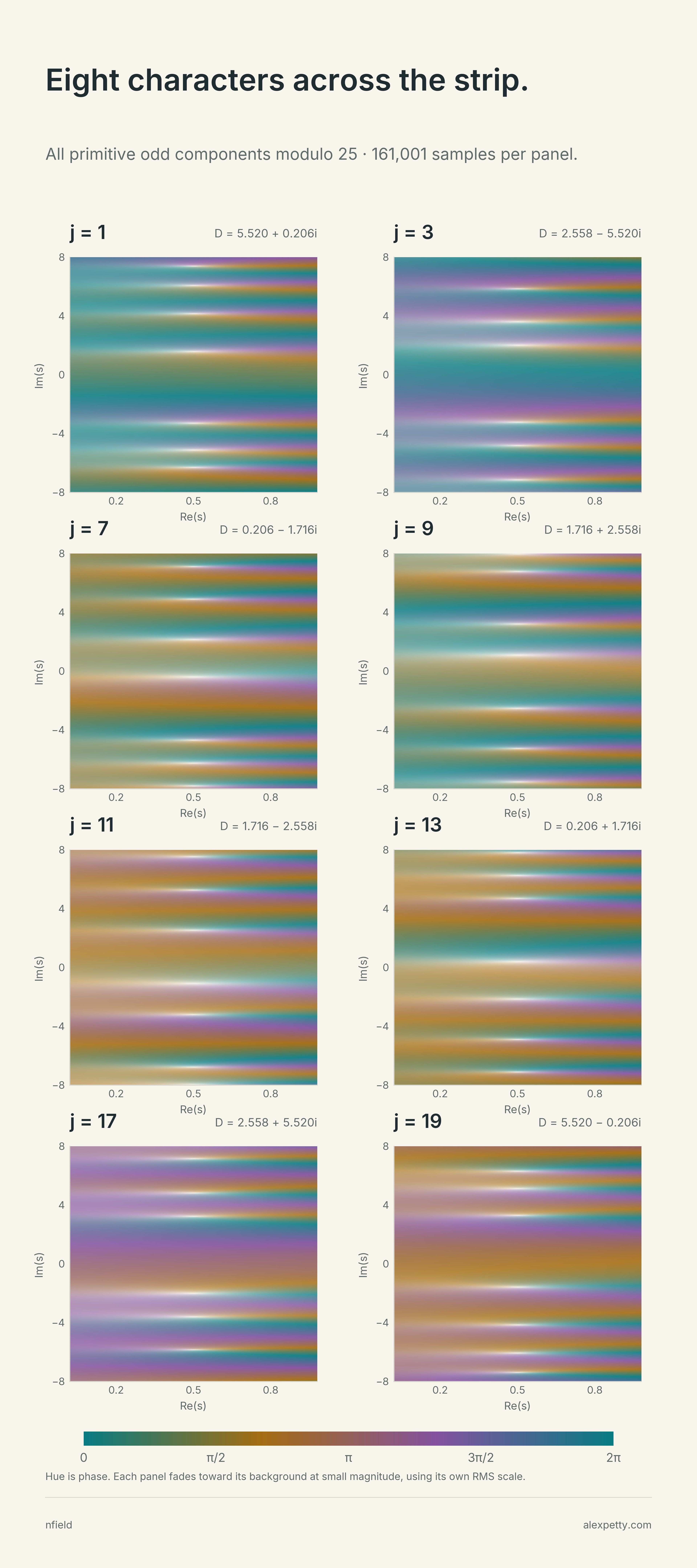
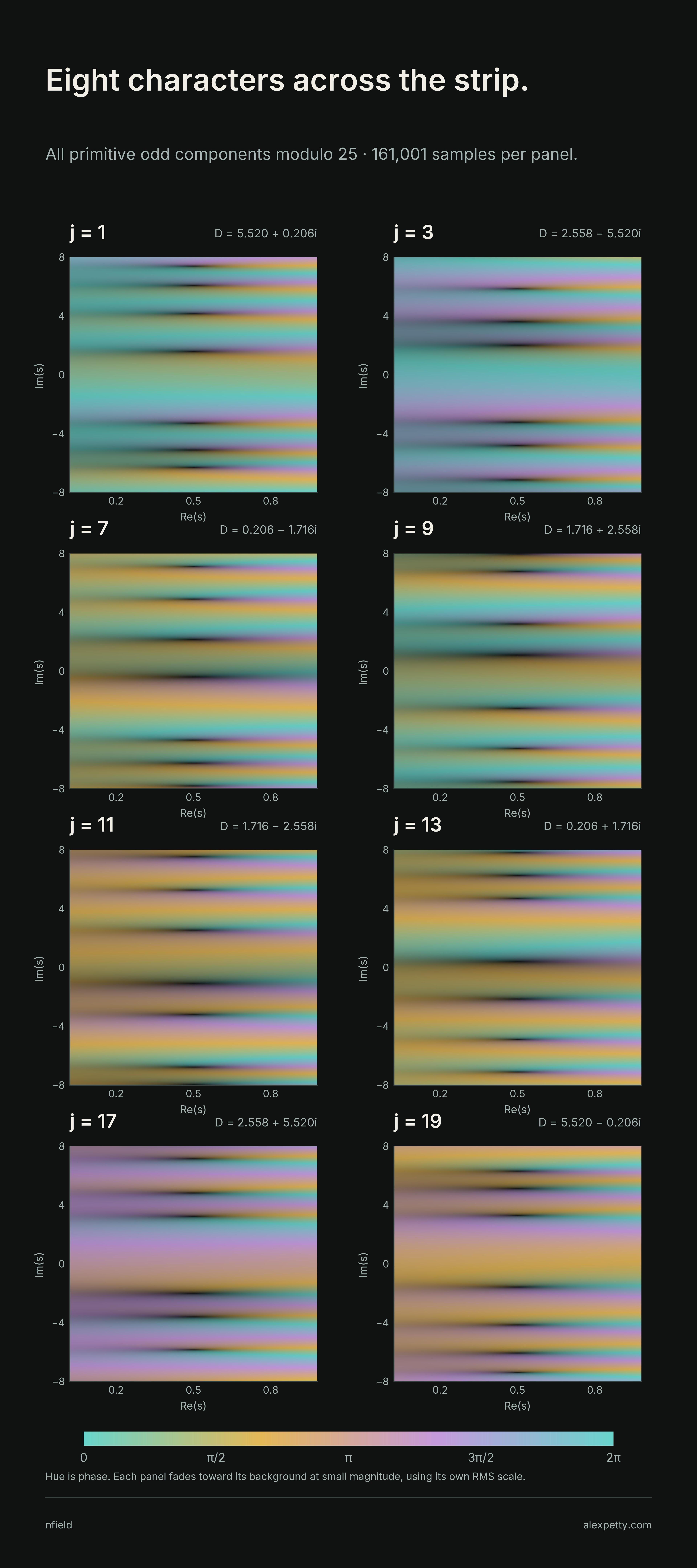
The numerical grid has $201$ horizontal and $801$ vertical samples per component. The direct kernel construction and its factored expression are checked separately. These pictures report finite computations.

This family is a different object from the prime-weighted series in The Collision Transform and the Critical Strip. There the complex parameter divides each prime’s weight, and here it enters through a kernel placed on a finite digit table. Identifying the two would take a separate argument.

The coefficient is waiting at zero

As $s$ moves to the left edge, the common factor tends to $i\pi/\varphi(m)$, and the classical value $L(0,\overline\chi)=-B_{1,\overline\chi}$ gives

$$\mathcal A_\chi(0)=-\frac{i\pi}{\varphi(m)} B_{1,\overline\chi}D_\ell(\chi).$$

At lag one in an odd prime base the right side is $i\pi$ times the finite collision coefficient, so dividing by $i\pi$ hands it back,

$$\frac{\mathcal A_\chi(0)}{i\pi}=\widehat S^\circ(\chi),$$

direction as well as length.

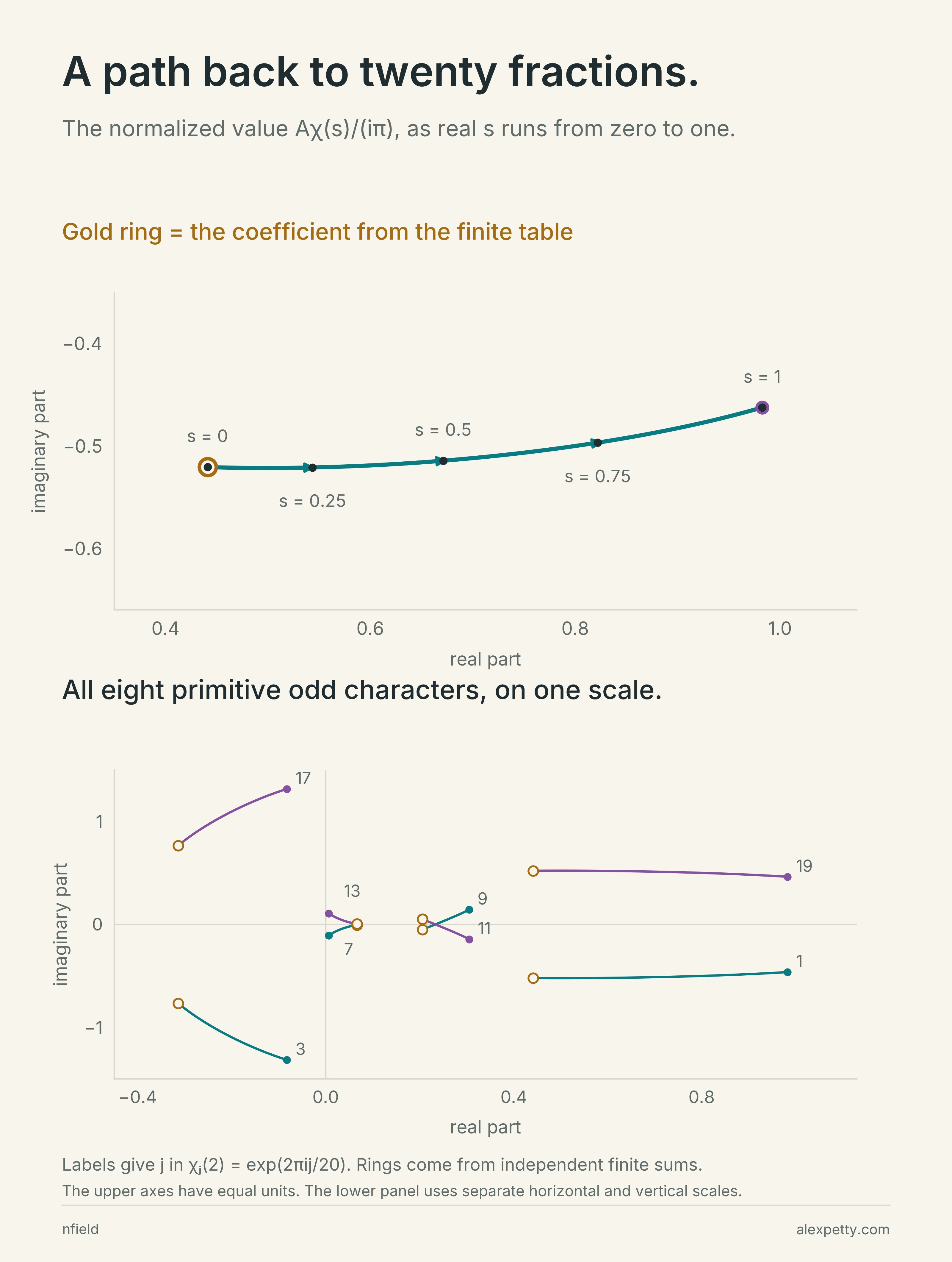
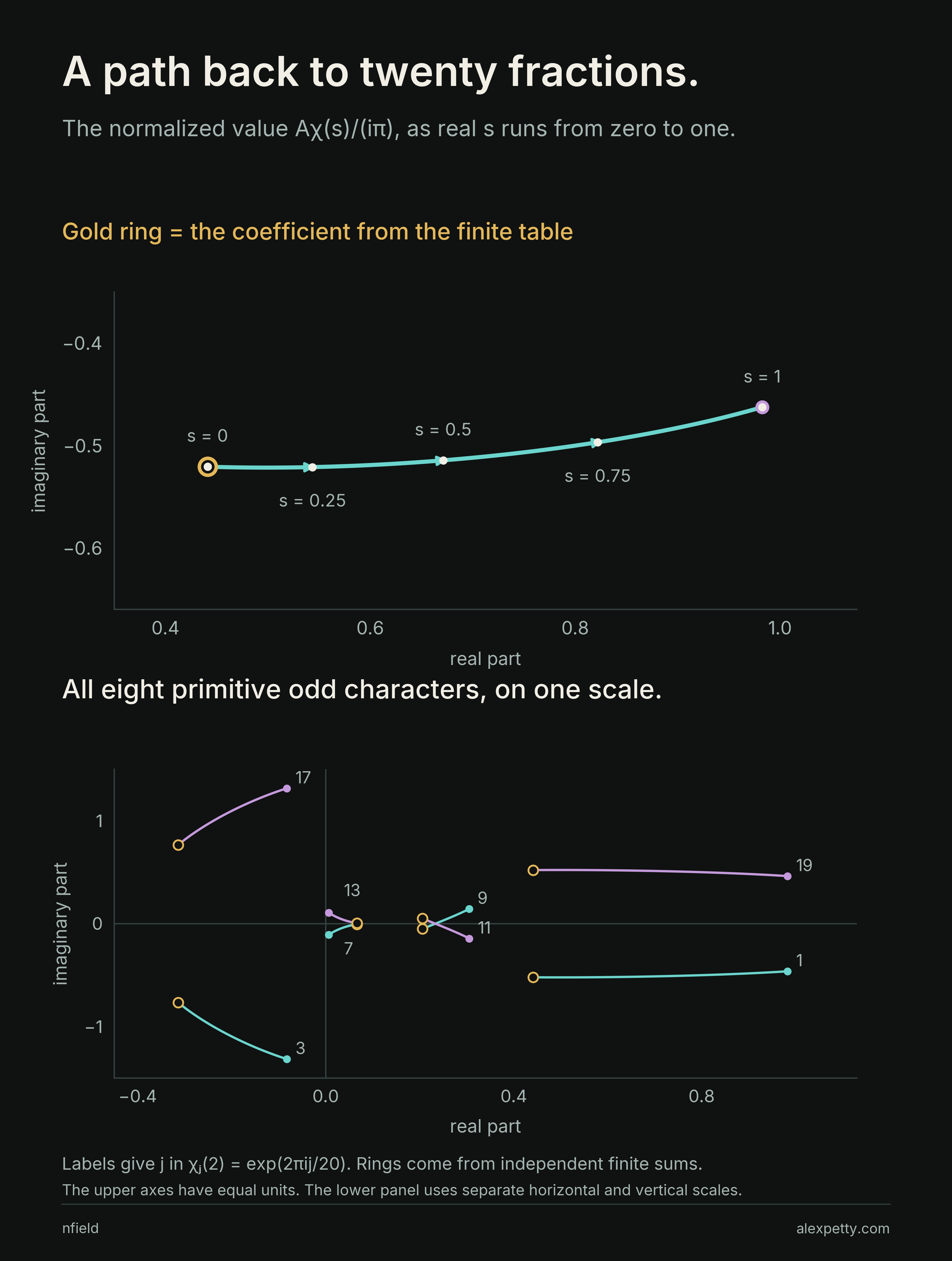
The top panel follows $\mathcal A_\chi(s)/(i\pi)$ as $s$ runs along the real axis from $0$ to $1$. It starts on the gold ring, which comes from averaging the twenty signed fractions directly, at about $0.441164-0.520524i$, and drifts right to $0.982604-0.462379i$ at $s=1$. No constant was adjusted to make the curve begin on the ring. In the lower panel all eight characters do the same, conjugate pairs mirrored across the real axis, each one starting from its own finite coefficient.

The far end is a different value. At $s=1$ the continued kernel is $-1/2+(i/2)\cot(\pi x)$, a Gauss sum enters the boundary formula, and the Bernoulli number switches from $B_{1,\overline\chi}$ to $B_{1,\chi}$. The Dirichlet functional equation connects the two edges without making them equal.

The two boundary formulas and all eight checks

With $B_{1,\chi}=m^{-1}\sum_{a\in U_m}a\chi(a)$ and the Gauss sum $\tau(\overline\chi)=\sum_{a\in U_m}\overline{\chi(a)}e^{2\pi ia/m}$, the right boundary is

$$\mathcal A_\chi(1)=-\frac{\tau(\overline\chi)}{\varphi(m)} B_{1,\chi}D_\ell(\chi).$$

Notice the change from $B_{1,\overline\chi}$ at zero to $B_{1,\chi}$ at one. Conjugation changes the phase. Keeping only magnitudes would conceal that difference.

Both columns below are divided by $i\pi$. The first also agrees with an independent finite-table calculation. Values are rounded to six decimal places.

Character exponent	At zero	At one
1	$0.441164-0.520524i$	$0.982604-0.462379i$
3	$-0.313818-0.765833i$	$-0.082709-1.314625i$
7	$0.066605-0.004988i$	$0.006675-0.106091i$
9	$0.206050-0.050296i$	$0.305440+0.143729i$
11	$0.206050+0.050296i$	$0.305440-0.143729i$
13	$0.066605+0.004988i$	$0.006675+0.106091i$
17	$-0.313818+0.765833i$	$-0.082709+1.314625i$
19	$0.441164+0.520524i$	$0.982604+0.462379i$

The grid, the fixed factor and the boundary curve, first drawings

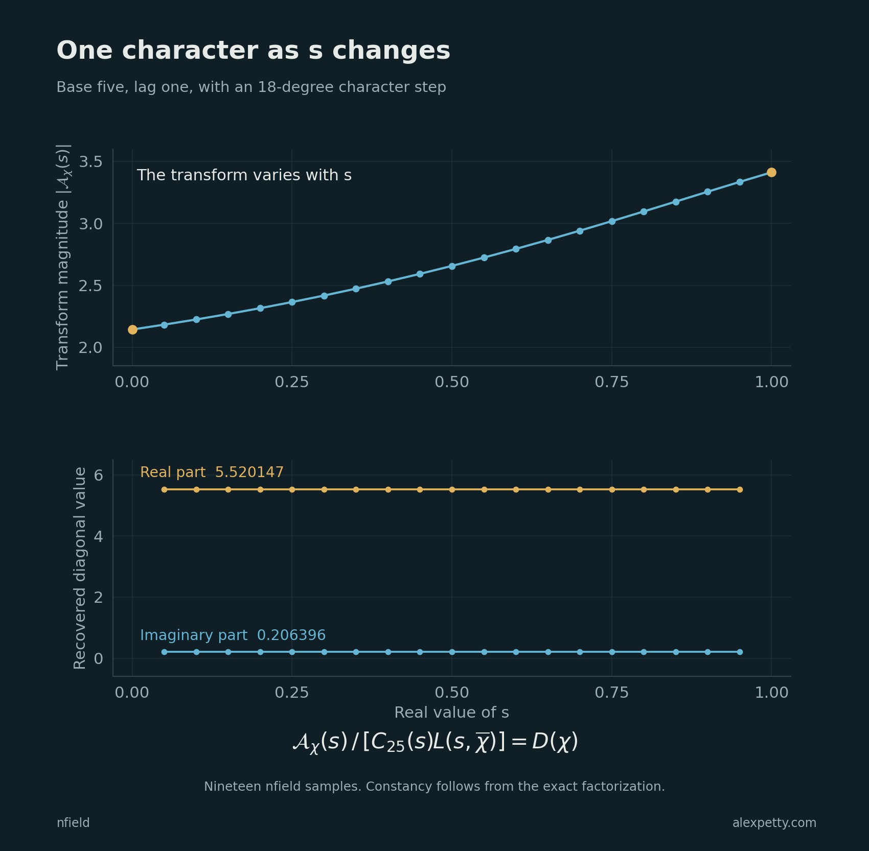
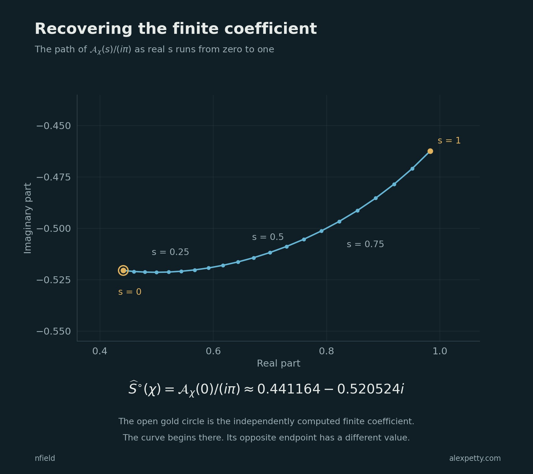
The factorization says nothing about where the zeros of $L(s,\overline\chi)$ lie, and it gives no estimate that holds as the modulus grows. It does fix the carrier exactly. For the eighteen-degree character at modulus $25$, the transform divided by $i\pi$ is $0.441164-0.520524i$ at $s=0$, the same number the twenty fractions give, and $0.982604-0.462379i$ at $s=1$.