Capacity
The Weight of a Carry
In 1861 Achille Brocot, a clockmaker in Paris, had a practical problem. He wanted gear trains that turn at awkward ratios, and he needed good fractions to approximate them. He found them with a single move. Between two fractions, put their mediant, the fraction you get by adding the tops and adding the bottoms. Between one half and two thirds goes three fifths. Keep doing it and every fraction in lowest terms turns up exactly once, in a tree. Moritz Stern had found the same tree three years earlier.
The remainder clocks in The Clocks Beneath Collision Energy, one for every period, carry weights. The two-position clock carries a quarter of the total, the three-position clock a sixth, four and five a twelfth each, six a thirtieth, and so on down, adding to exactly one. The shares look arbitrary. Nothing about a clock that turns forever suggests it should weigh a thirtieth, and conservation alone cannot explain them, since any shares adding to one would keep the clocks turning.
They come from Brocot’s tree. Every gap between neighboring fractions in the tree pays a share to exactly one clock, the clock whose period is the denominator of the fraction that will split that gap. The gap from zero to one pays the two-position clock its quarter. The two gaps on either side of one half pay the three-position clock a twelfth apiece. And the payments are made by the carry, the digit you move into the next column when a sum overflows, because a carry splits things exactly the way the tree does.
Three plus three on a clock of five
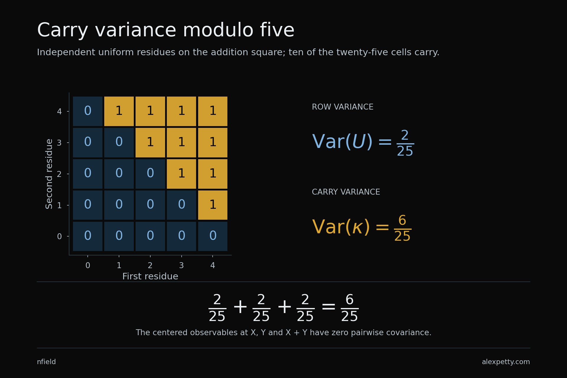
Start with three plus three. On a five-position clock, six becomes one and leaves a carry. Double every position and the carries are zero, zero, zero, one, one.
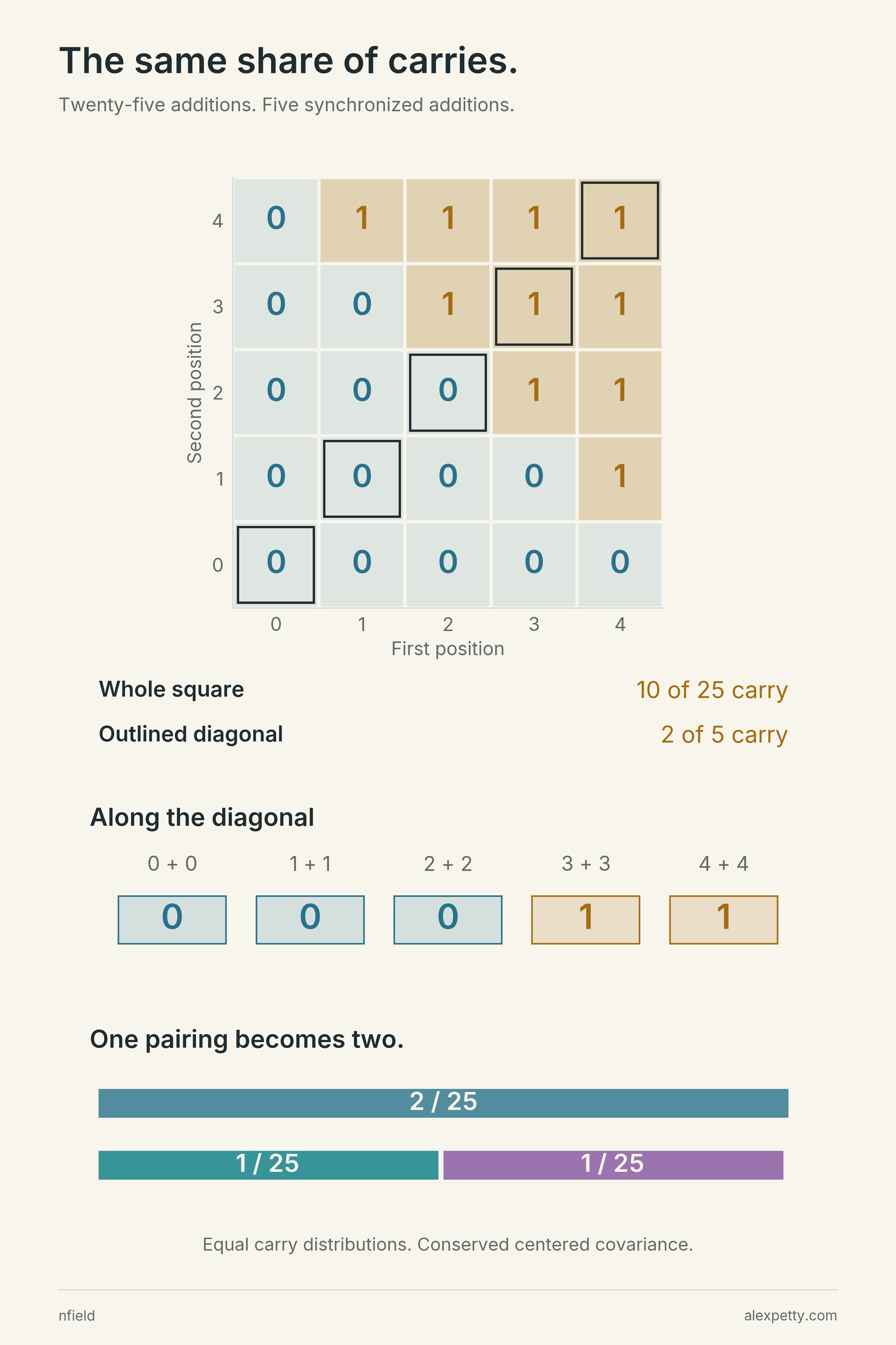
The full addition square has twenty-five cells. Ten carry. The five cells along its diagonal have two carries. Both experiments give the same two-fifths share, even though the diagonal ties the two inputs together.
That small agreement has a consequence. Measure how the centered rows vary together. Replacing a pair of rows by its two children, each paired with their sum row, divides the original measurement exactly. In this example, becomes .
Here the parent compares the original row with itself. Each child compares that row with the doubled row, in opposite orders.
The pairing survives while the rows themselves move on.
Look at the labels on those rows. The pair (1, 1) splits into (1, 2) and (2, 1). Wherever the rows make sense, a pair (a, b) splits into (a, a + b) and (a + b, b), and nothing is lost in the split. That is Brocot’s move, made by a carry.
The carry and the conserved pairing
At modulus , use the centered residue row
Assume , and are all units modulo . Each row then has variance .
On the full addition square, the two inputs and their reduced sum are pairwise independent and uniform. Their centered signed sum is the centered carry. Its variance is therefore .
On the synchronized line , the carry is still zero or one and has the same mean. Its variance must also be . Expanding that variance gives
Independence belongs to the full square, not to the synchronized line. The line’s rows are dependent. Their covariance is what the identity preserves.
Twice as big, four times the cost
Capacity measures the average squared size of the collision response. Could another rule do the same job?
The paper makes the question precise. Give each centered value its own cost, using one continuous, even rule at every scale. Average those costs. Require the pairing formed from sums and differences to obey the carry split.
The rule is forced to be a constant times the square. Doubling a value must multiply its cost by four. A five-position test also forces tripling to multiply it by nine. Continuity leaves no room between those requirements.
This depends on measuring values individually. A rule that combines the whole row first can escape it. The theorem keeps that assumption in view.
The precise measurement test
For a continuous even density with , define
and
Carry refinement is required for all real amplitudes and all unit triples at every odd modulus. The root triples at growing moduli give . The root triple at five gives . The quotient , viewed on a logarithmic scale, has the two incommensurable periods and . Continuity makes it constant. Nonnegative, nonzero cost gives a positive constant, and one variance calibration makes it one.
The nonlocal rule also passes the unit-row carry tests. Thus carry refinement alone does not select squared size among every conceivable measurement. Nor does one five-entry table prove the all-amplitude theorem.
The digits supply the rows
In base five, the equal-digit cells are 00,
11, 22, 33 and 44.
Count their boundary crossings and subtract the baseline. Reorder the
twenty-five phases by the digit rule. The resulting values lie exactly
on a sum of four rising, resetting waves.
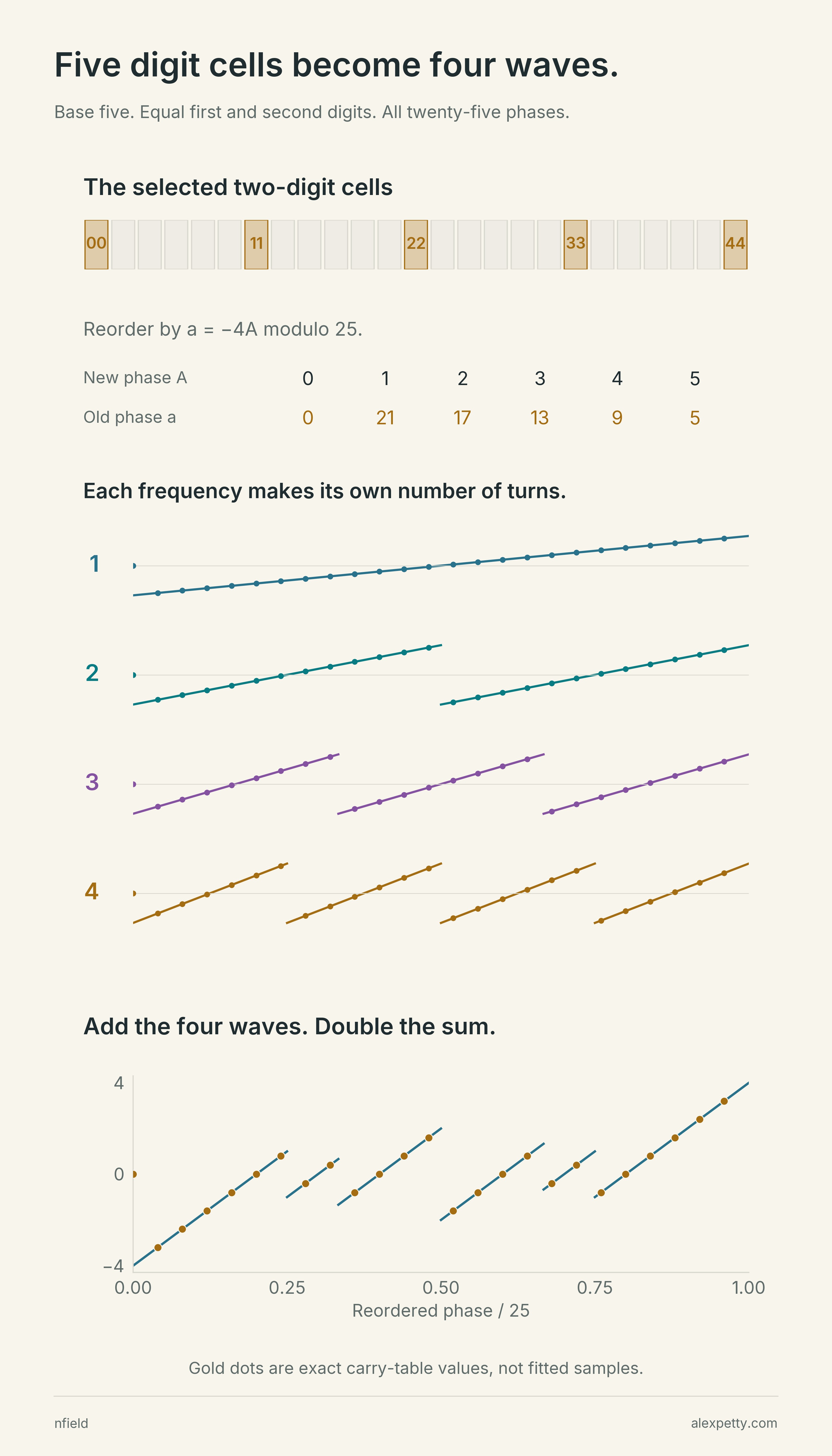
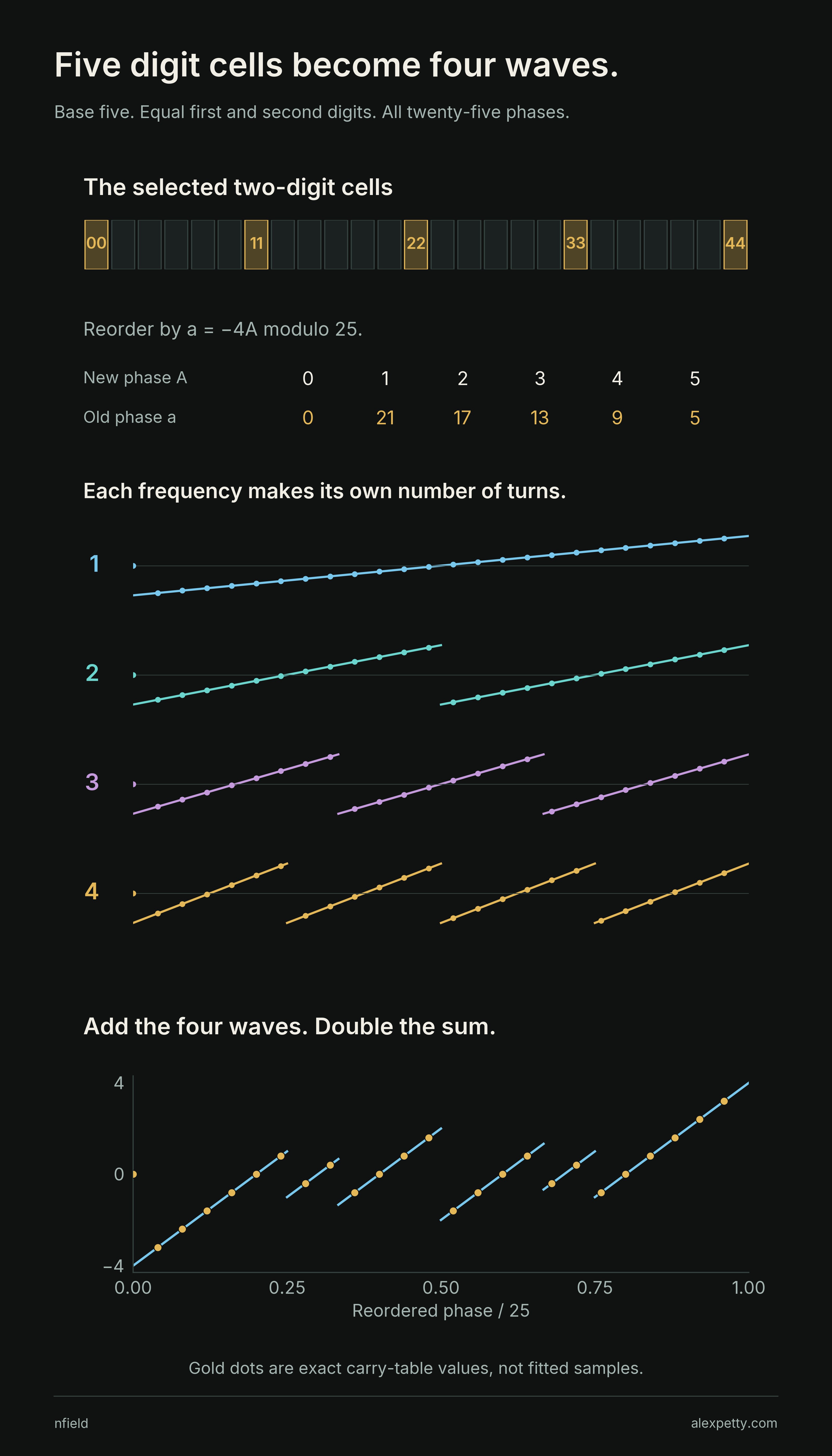
The waves make one, two, three and four turns. There are no skipped frequencies or adjustable coefficients. The digit condition supplies them.
This straightening works in every integer base and at every two-position lag. The row labels must stay attached. They tell us when each contribution first enters as the calculation grows.
The exact straightening, including the endpoints
Let be the base, the lag, , and . The equal-digit cells are
Their centered table is
Write off the integers and zero at an integer. The exact identity is
At base five and lag one, the phase multiplier is . All twenty-five phases, including zero, are retained in the figure. The plotted ramps are the prescribed affine functions, not an arbitrary interpolation between those samples. Their continuous capacity is
The finite sampled energy and this integral are different quantities. Their comparison requires an additional sampling estimate.
There is also an endpoint correction between ordinary centered residue rows and sampled midpoint sawteeth. For unit frequencies,
where . Omitting it leaves a refinement defect , equal to at five. The paper retains the correction before passing to the affine pairing. Higher-lag nonunit rows are covered by straightening, not by this unit-row endpoint formula.
Every gap pays a clock
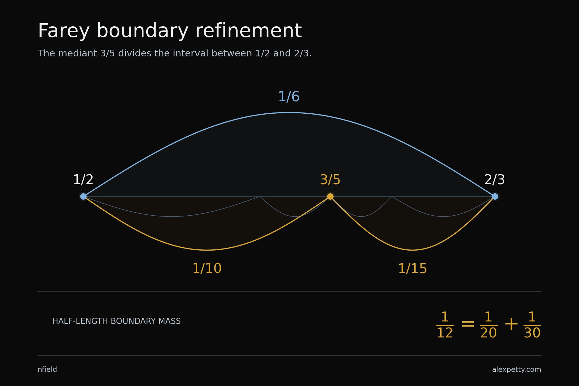
Now the tree itself. Mark one half and two thirds, neighbors in Brocot’s tree. The gap between them is one sixth. Insert their mediant, three fifths, and the gap splits into one tenth and one fifteenth. Nothing is lost.
The continuous pairing assigns half the gap to its boundary. So divides into .
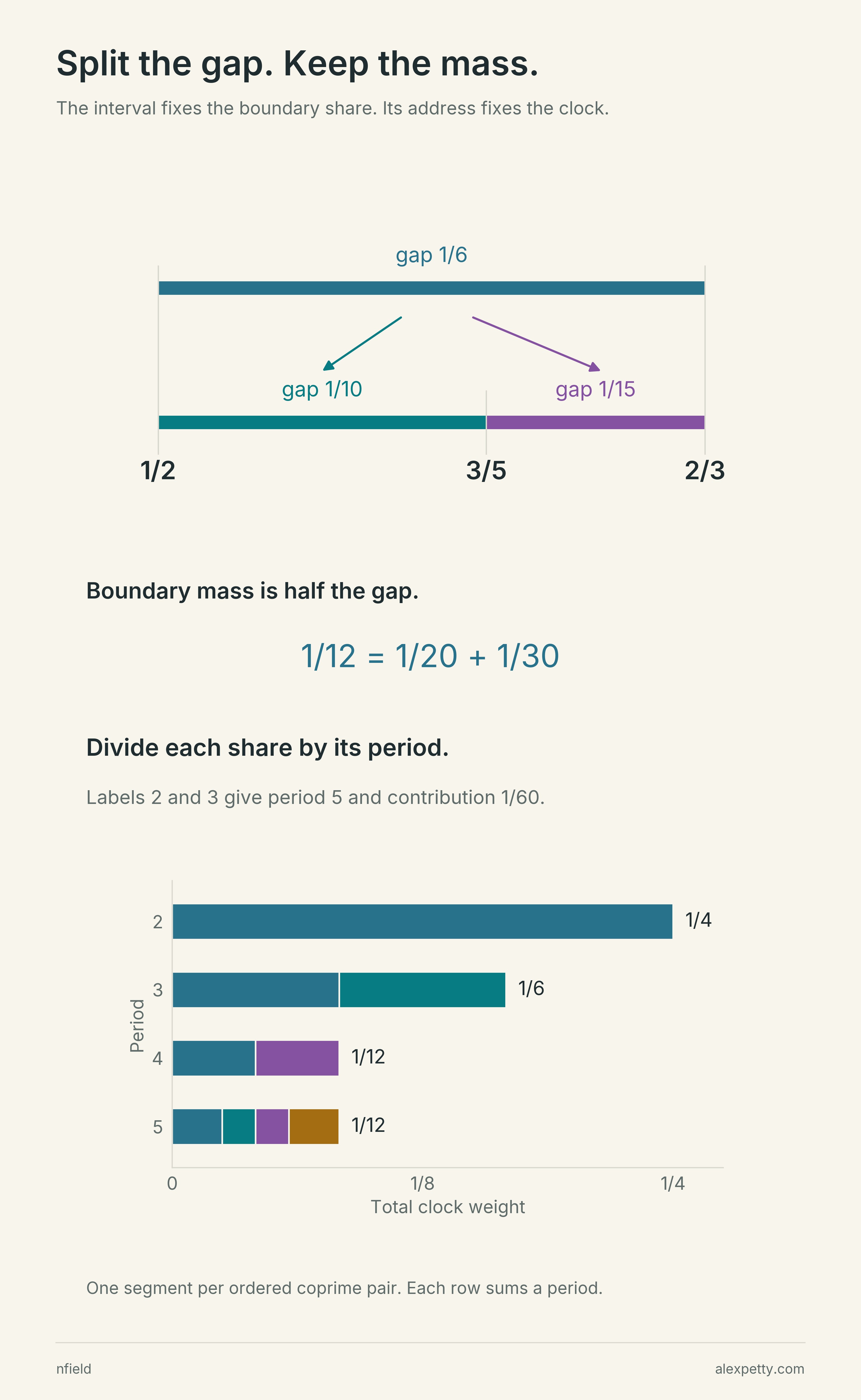
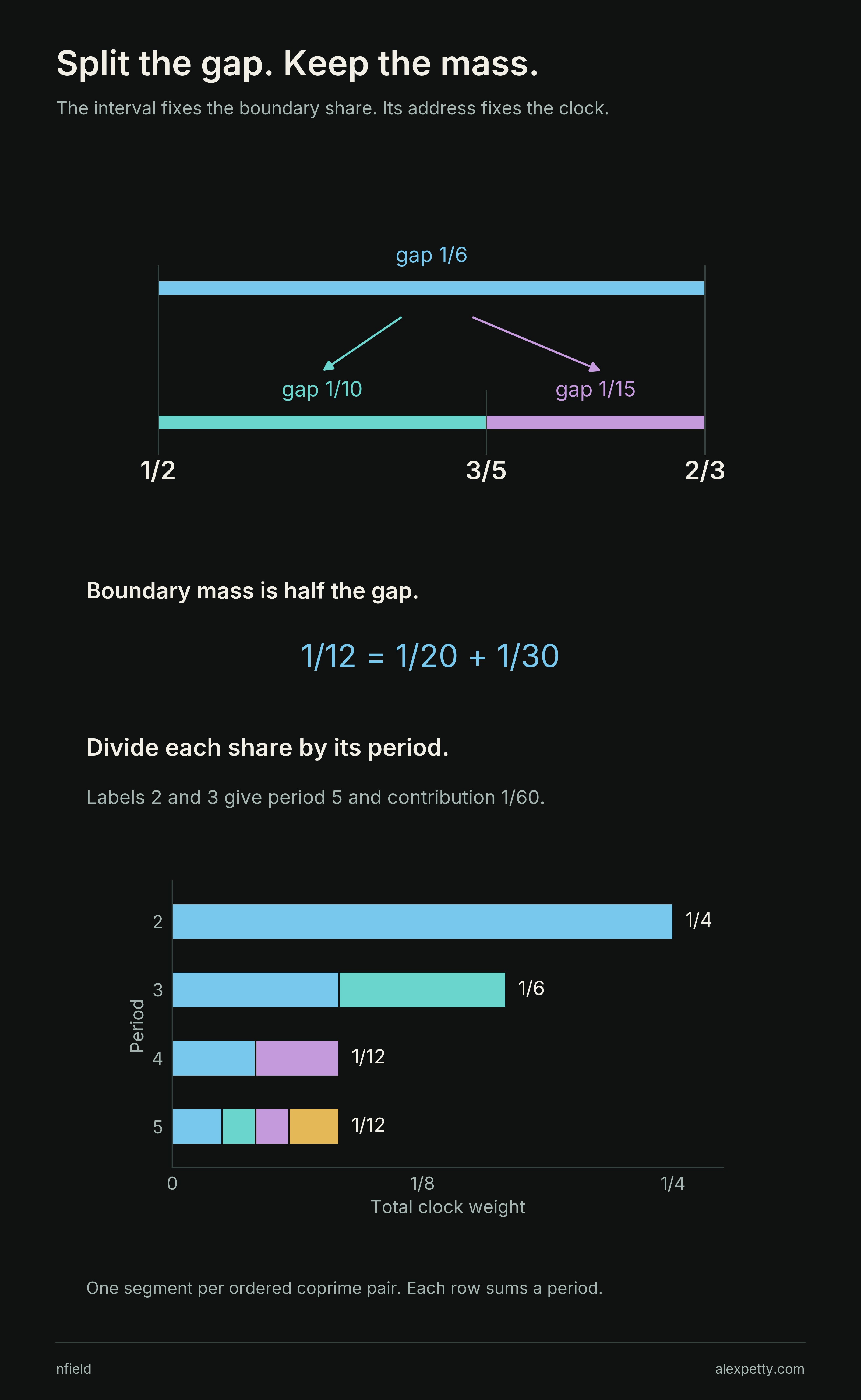
To turn that boundary share into a clock weight, divide it by the denominator of the mediant, the sum of the two denominators at the ends of the gap. The gap from one half to two thirds splits at three fifths, so its share of pays the five-position clock .
Every clock collects from every gap whose mediant has its period as denominator. Counting every gap in the tree supplies all the weights, and a telescoping sum down the tree proves they add to exactly one.
Boundary mass, period mass and the conserved unit
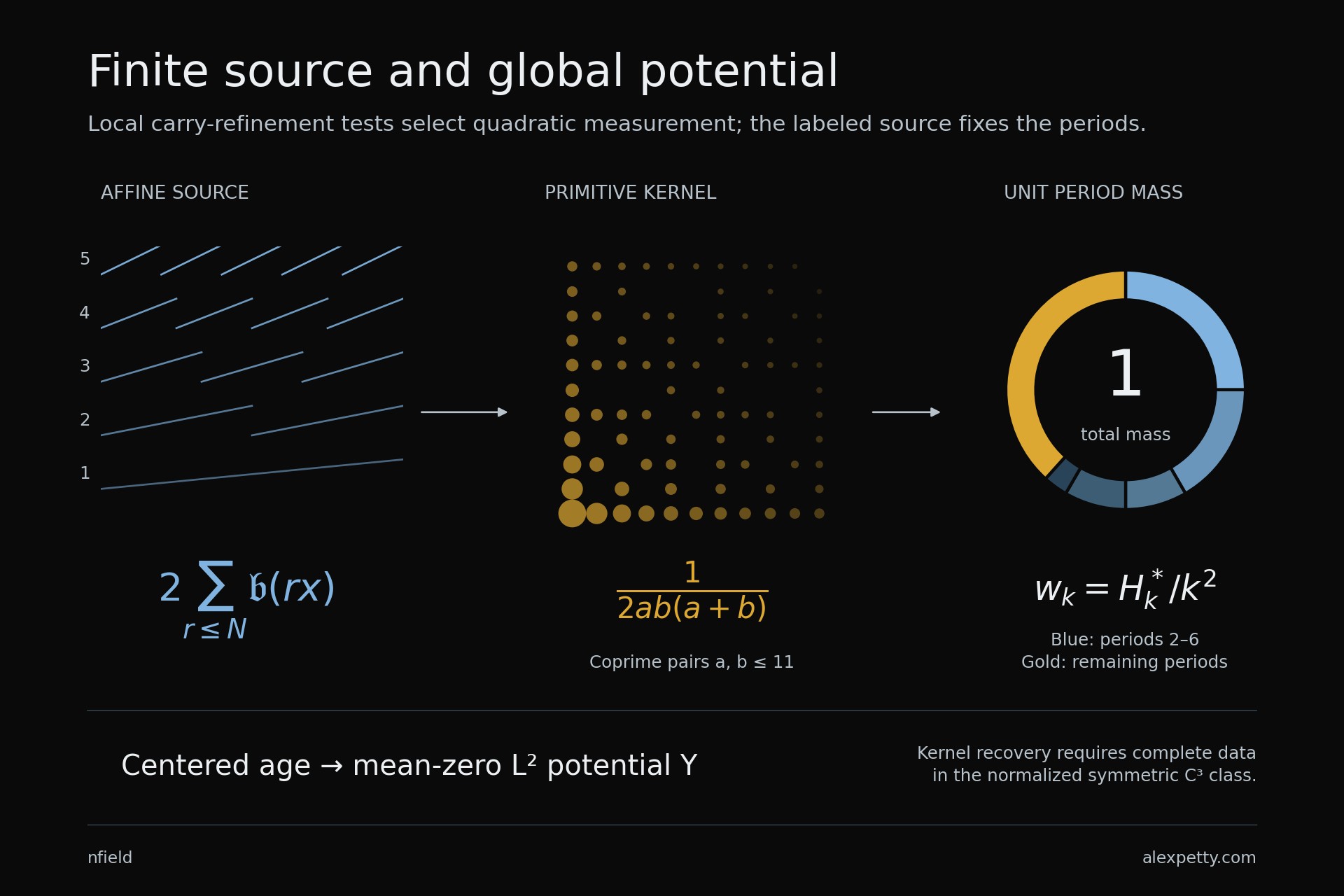
For coprime positive , the affine covariance is . The paper’s normalization makes its boundary mass
It obeys . This is the conserved half-length under classical Farey subdivision. The clock contribution is a different quantity,
Its period sum is
The calculation first admits a reduced pair at cutoff . Larger cutoffs contain common-scale copies. Those labeled appearances force the address, which conservation by itself cannot do.
The reciprocal kernel follows directly from the paper’s ledger. It also has an independent uniqueness characterization. Among symmetric degree-minus-three kernels with a continuous normalized angular profile, conservation of the period-weighted boundary under this same subdivision forces the reciprocal form. Unit total mass fixes its constant. The unweighted clock contribution is not what adds under an individual Farey split.
Run the calculation backward
A capacity compresses the whole wave into one number. That invites a question Mark Kac made famous in 1966, when he asked whether you can hear the shape of a drum, whether the tones a drum makes determine its outline. For drums the answer, found in 1992, is no. Here the capacities are the tones. Keep one at every resolution and the compression can be run backward.
The first four capacities are , , and . Each individual doubled wave contributes . Subtract those individual contributions, rescale, and compare successive totals. Each difference contains the weights of the clocks resetting at that integer.
At four, the two-position clock resets again. Its weight is already known from two. Subtract that contribution and the remaining increment reveals the weight at four.
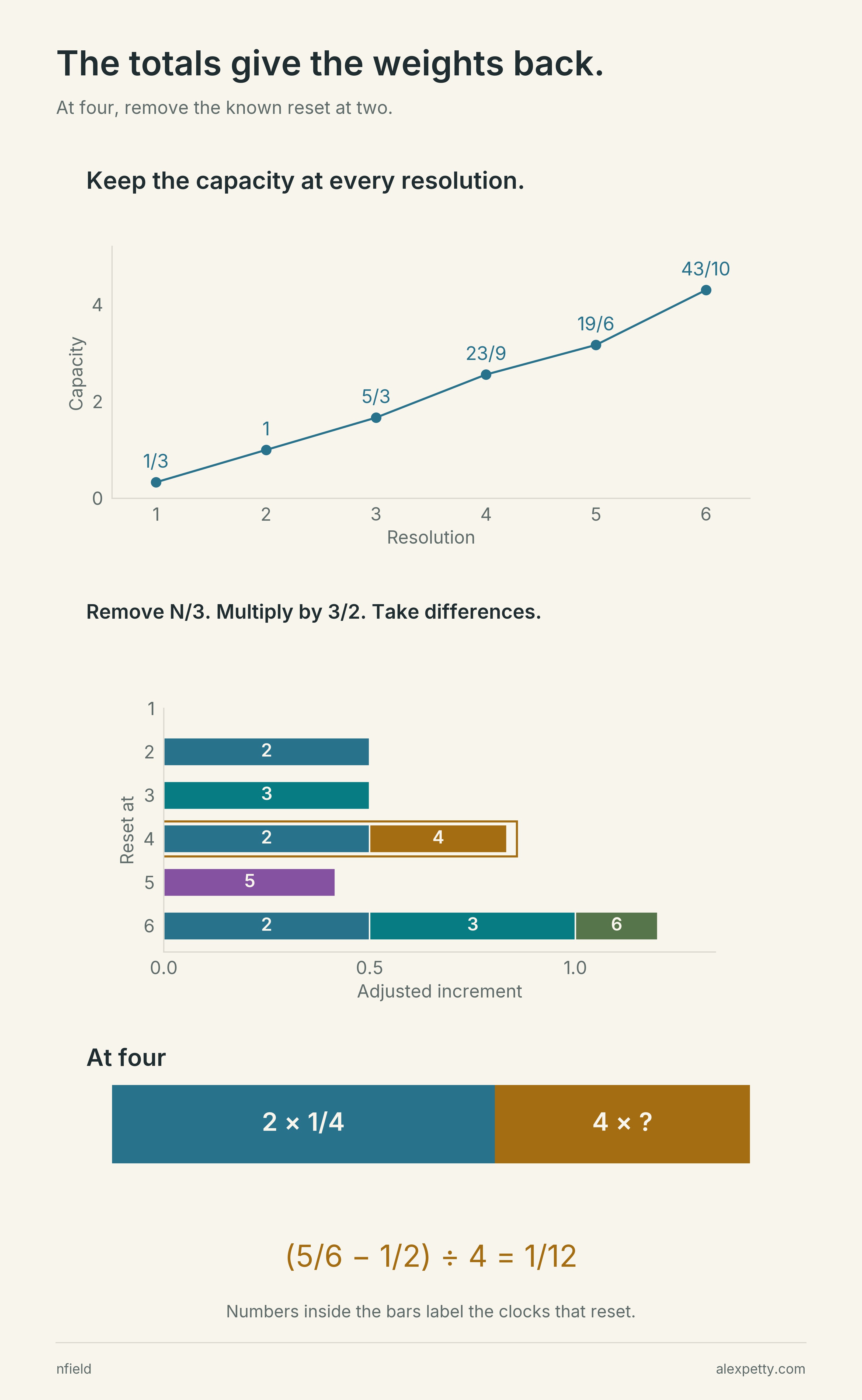
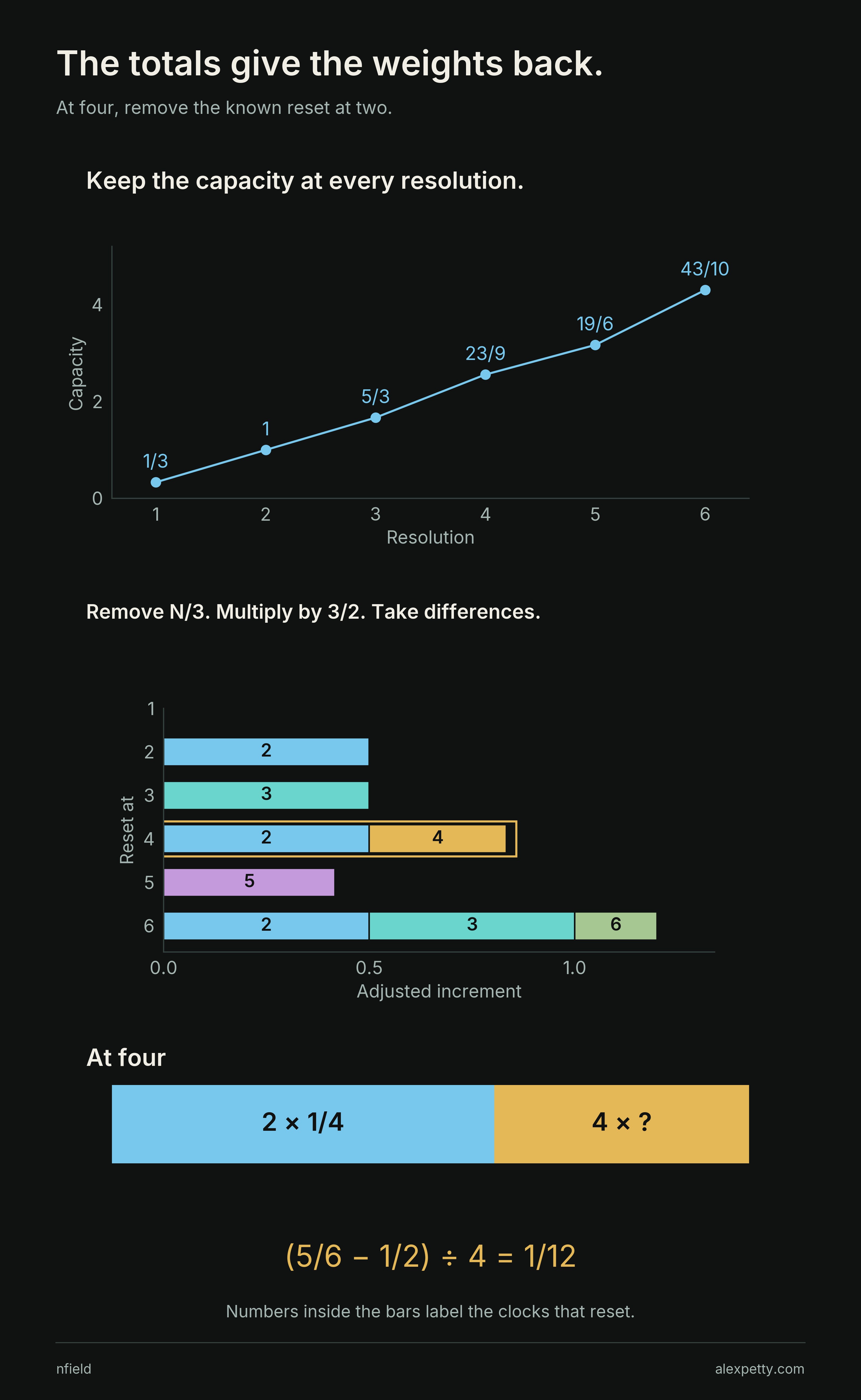
Continue and every new resolution exposes one new weight. Within the paper’s smooth symmetric boundary class, the entire sequence then recovers the boundary profile itself. It does not recover an arbitrary realization of the original digit tables.
The inverse, with six exact entries
Expanding the square gives from the individual waves. The cross-pair terms have a common factor . Remove the former and divide by the latter. This gives , with . Its differences obey
This is a triangular recovery. Every proper divisor is smaller than . Subtract its known contribution and divide by .
| Resolution | Capacity | Reset increment | Recovered weight |
|---|---|---|---|
| 1 | |||
| 2 | |||
| 3 | |||
| 4 | |||
| 5 | |||
| 6 |
In particular,
For the kernel inverse, write
The theorem assumes a symmetric profile, positive inside the interval, with unit total primitive mass. Divisor inversion restores full grid sums from primitive sums. After removing the endpoint singularity, grid averaging and Fourier inversion recover the profile. This step needs the complete infinite sequence and the stated regularity.
Symmetry is essential. An antisymmetric perturbation cancels inside every period sum. Fixed phase coordinates are essential too. Translating all waves leaves their squared integrals unchanged but moves their boundaries. The theorem recovers the regular symmetric primitive ledger, not unrestricted source data.
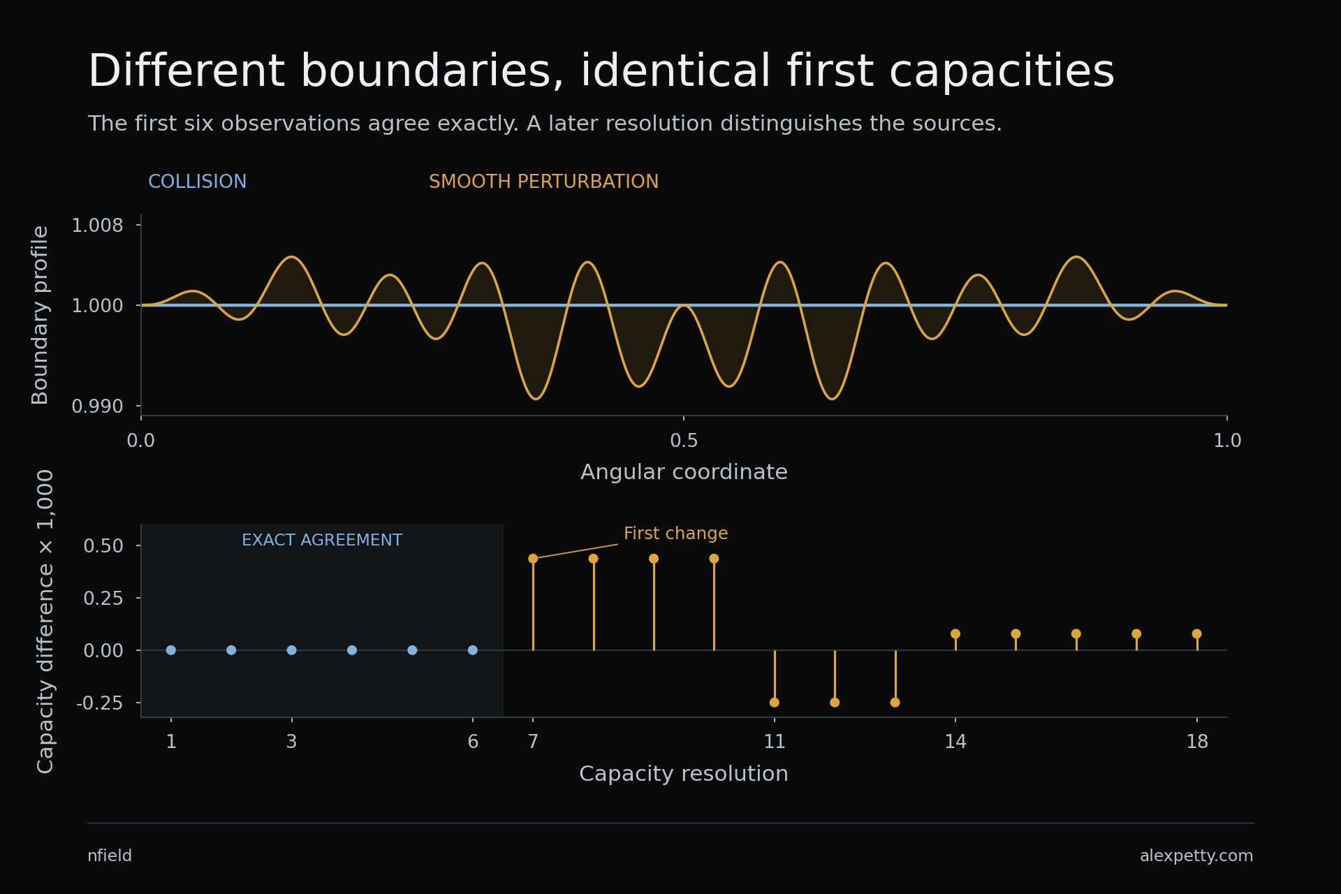
Six identical answers
Stop at six. Two different boundary rules can give exactly the same six capacities. No rounding, no measurement error.
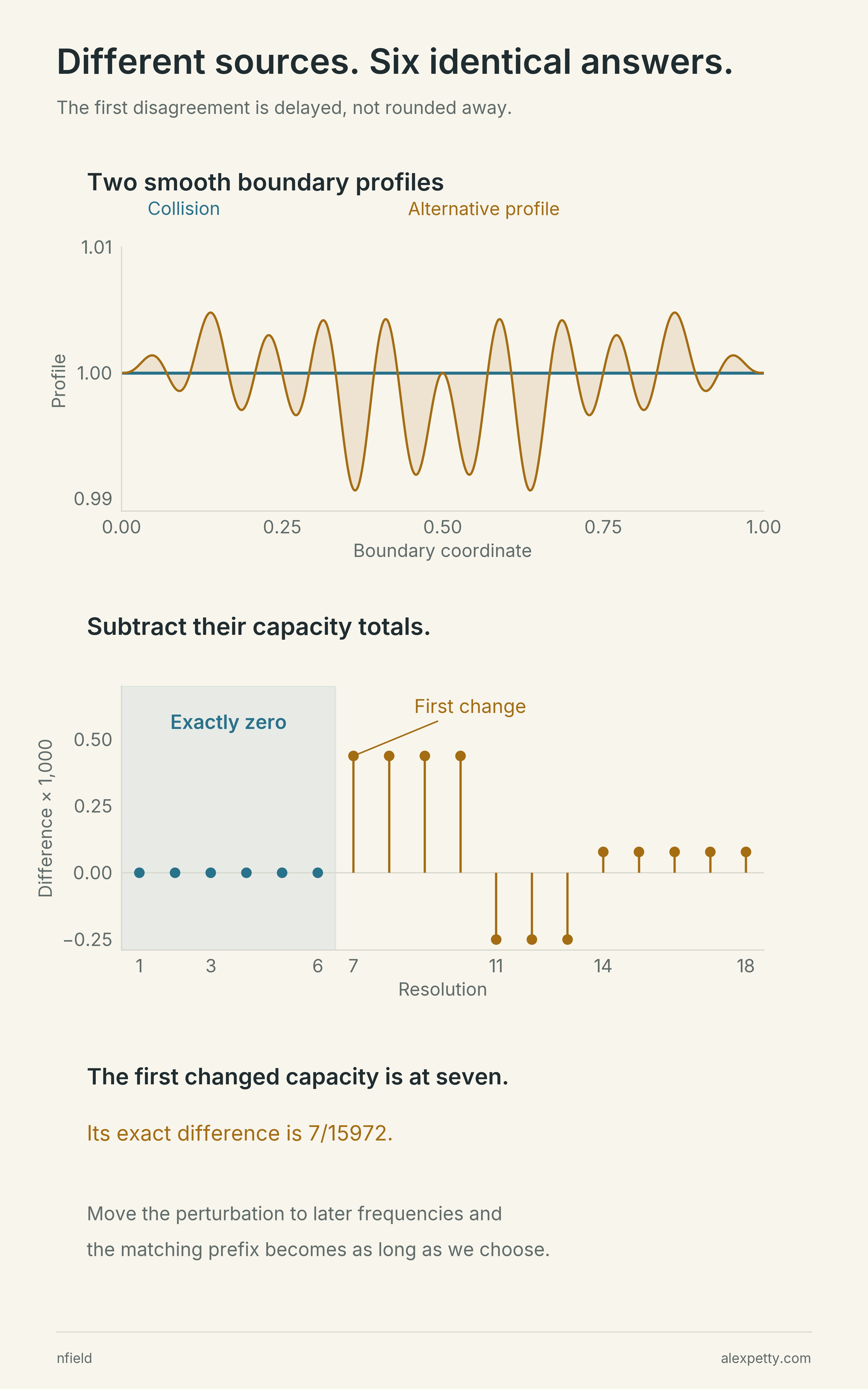
The blue profile is the collision rule. The gold profile is a smooth positive alternative. Their first disagreement appears at seven. The construction can put that disagreement beyond any finite cutoff we choose.
The full record identifies the boundary, and no finite record can.
Exact recovery is not cheap recovery either. The paper gives a signed readout of the weights that returns at every prime power and zero everywhere else. Nothing in its definition mentions a prime, and the primes come out of the carry weights anyway. It proves nothing new about primes, but it is a strange place to meet them. The readout’s sensitivity at the first changed address grows like , so a small change in the whole state can become a large change in a late coefficient.
The hidden perturbation and the sensitive readout
The displayed control uses primes , and . Set
and . The profile is symmetric, smooth and positive. Its primitive mass remains one. Grid averaging makes its unprimitive rows differ only at seven and eleven. Finite divisor inversion gives the exact changes of period mass and capacity. The first capacity difference is at seven.
For the signed readout, first form the angular row
Normalize its adjacent differences by , so . Logarithmic marking and Dirichlet convolution inversion define
For the collision weights, . The classical identity then gives . The whole current recognizes the collision mass. This supplies no new prime-distribution estimate.
The control first changes the normalized increment at six, one step before the first changed capacity. Its current there is , while the collision current is zero. The sharp sensitivity concerns a growing first changed address, with preceding increments and the scale held fixed. It does not say that a fixed coefficient is discontinuous or that signed sums cannot cancel.
The primitive pairs, from twelve to seven hundred sixty-eight
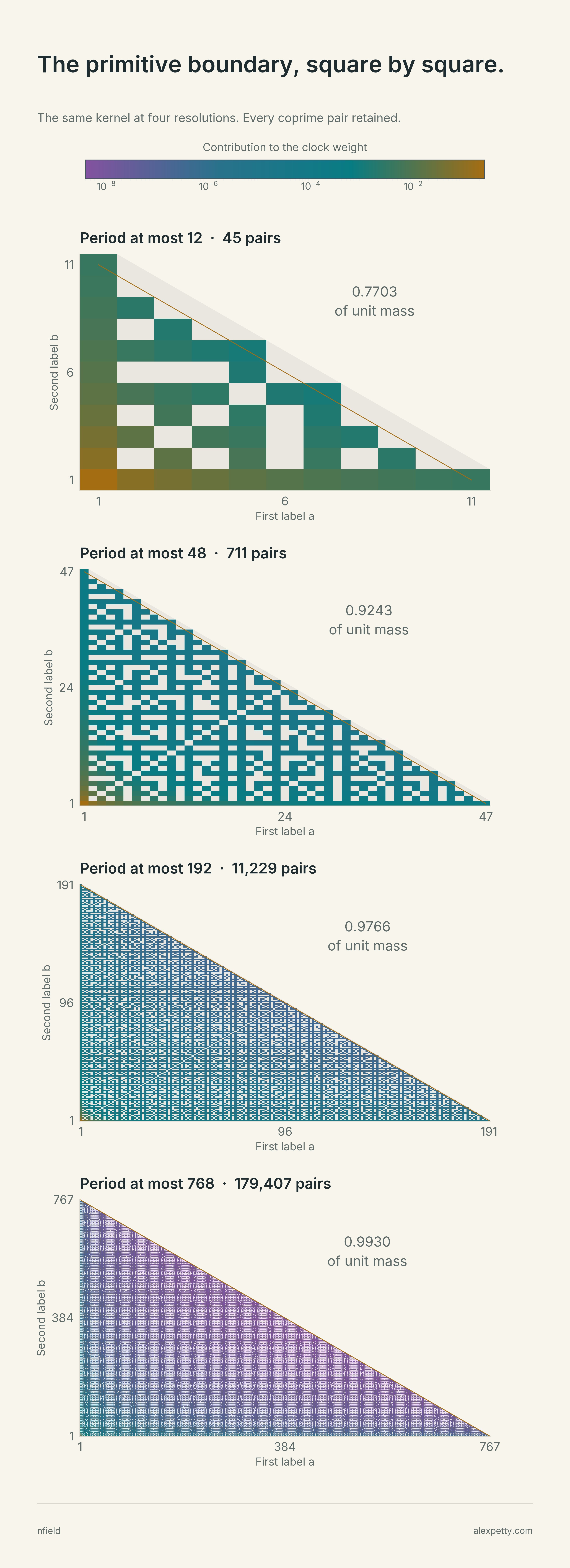
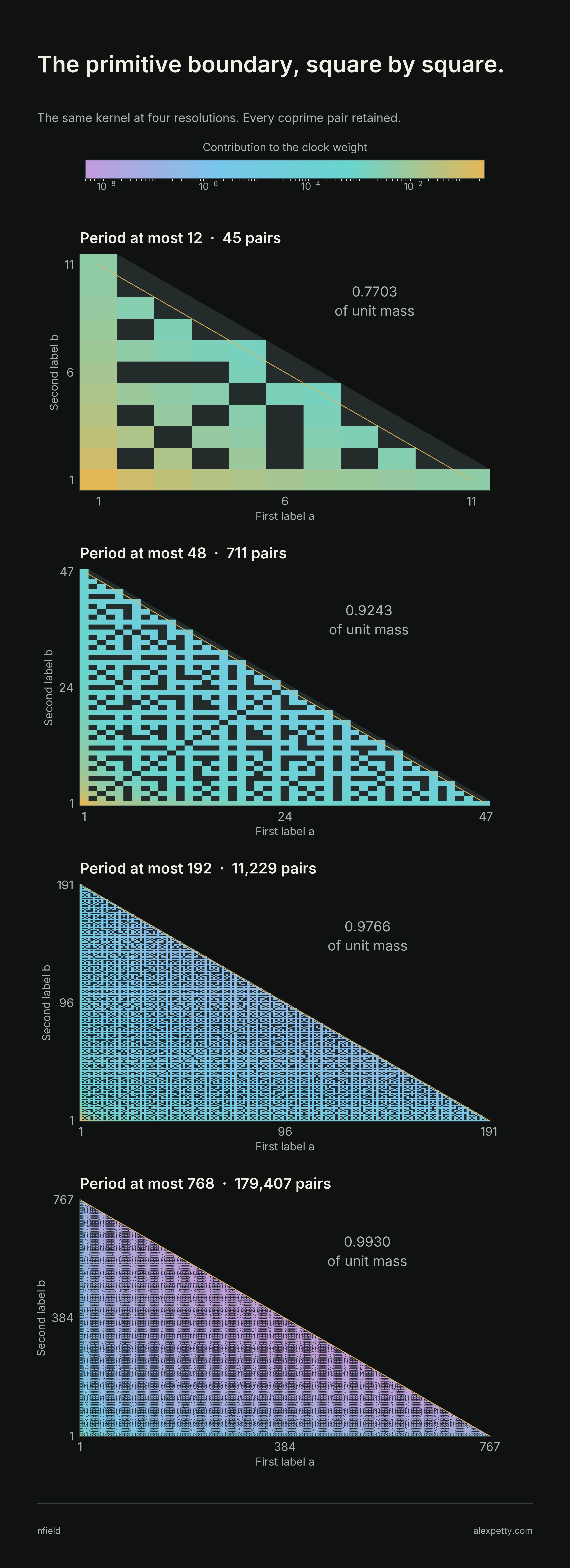
Every occupied square is a coprime pair. Its diagonal address is the period . Colors show the actual kernel contribution on one logarithmic scale across all four panels. The gaps are pairs with a common divisor. All cells are retained. These are the individual contributions whose period sums give the clock weights.
Four close studies of generation and recovery
The full proofs are in Finite Generation of Collision Capacity.
Six answers can agree exactly and come from different boundaries. So can six million. The construction lets me move the first disagreement past the last number you have checked.
Discussion
Sign in to join the discussion.