The Bias Beneath the Secondary Term

The Clocks Beneath Collision Energy ends on a strange mystery. Its clock model behaves perfectly on average, over every way the clocks could be set. But the integers, the numbers we actually count with, are a sliver of those settings, so thin that the average cannot see them. At every one of them the model’s readout runs off to minus infinity. The whole is calm, and the part we live in falls without end. Why should the numbers we actually use be the one place the model breaks?

The answer is in how the real calculation reads its clocks. It never holds the collection fixed. At integer $n$ it reads every clock through period $n$, so each step brings in one new clock, and every new clock starts at the bottom of its cycle. A clock that has not finished its first turn has spent all its time below average. Those unfinished turns drag the readings down, a little further at every step, by about a thirtieth of $\log n$. Remove that drag exactly, and the readings over long stretches of integers fall into the clock model’s distribution after all.

The same thing happens twice more. Read only at the integers just below primes, and the average drops by exactly one third. Hold the collection of clocks fixed for a stretch, and a parabola appears in the data. In all three cases the effect comes from the way the readings are taken, not from the numbers being read, and each one has an exact formula. Take them out, and the readings show the fluctuation the clock model was describing all along.

Clocks that arrive at the bottom

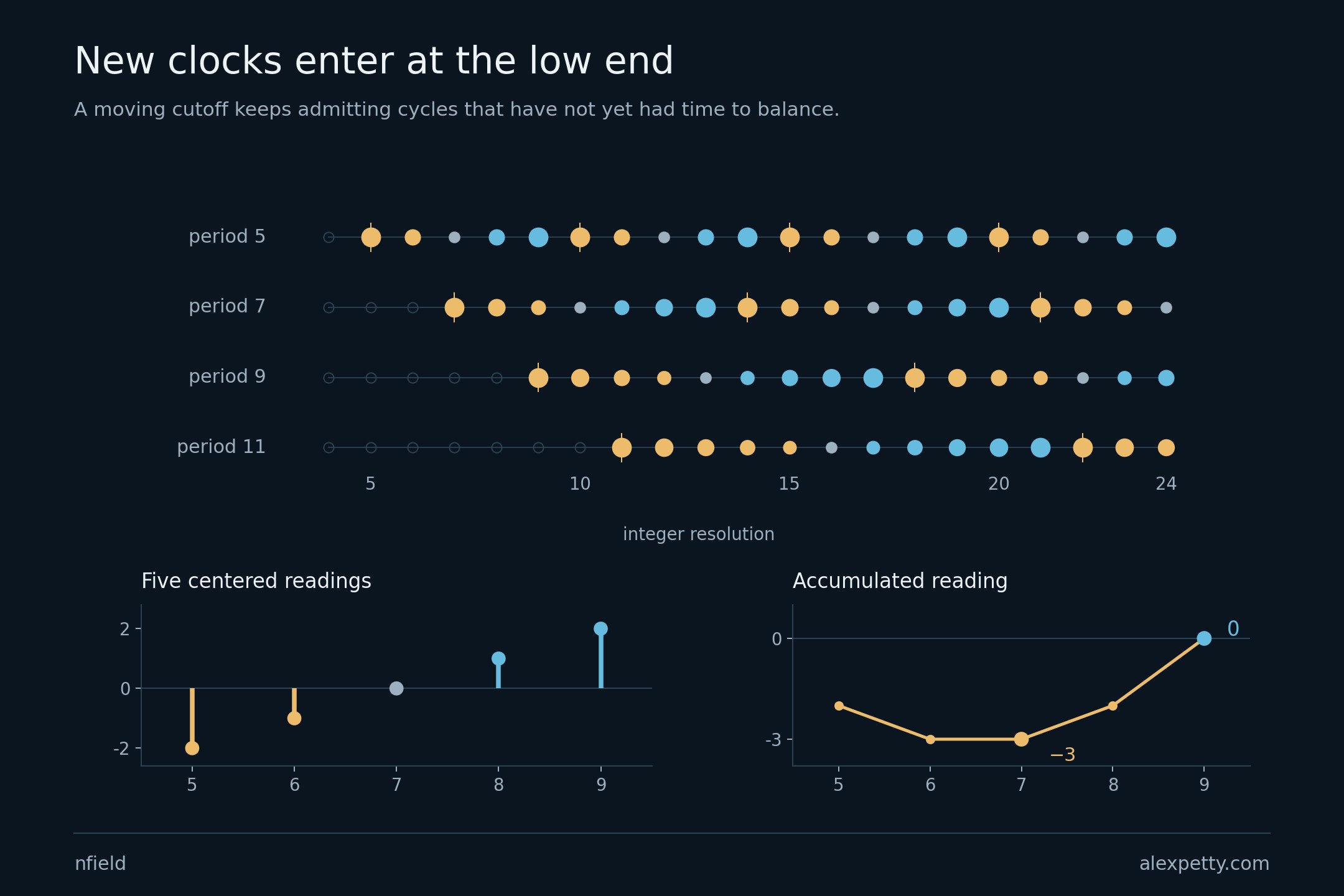
The drag can be seen in a single clock. A period-five clock reads zero, one, two, three, four, then starts again. Subtract its average, two. The five readings become

$$-2,\quad -1,\quad 0,\quad 1,\quad 2.$$

They add to zero. But the calculation admits this clock at integer five, just as its hand returns to zero. Through integer seven, we have collected only the first three centered readings. Their sum is minus three.

At nine, the clock pays back the difference. By then, the clocks of periods six, seven, eight and nine have joined the calculation. Each arrives at the bottom of its cycle.

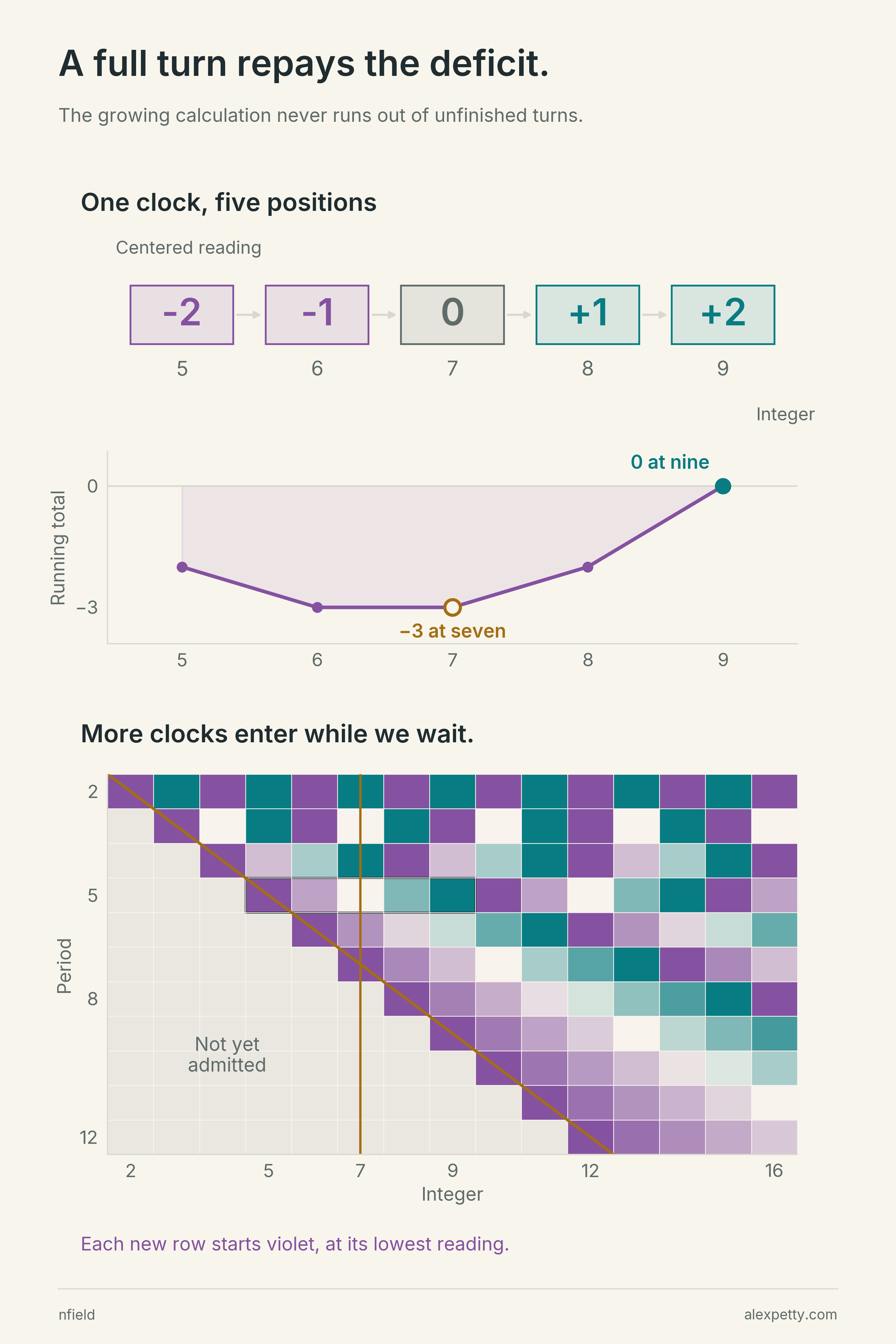
Each clock carries a positive weight fixed by the arithmetic. A complete turn contributes nothing to the accumulated centered reading. An unfinished turn can only leave a deficit.

There is always another clock arriving.

The exact clock ledger

For period $k$, write $r_k(n)=n\bmod k$ and

$$w_k=\frac1{k^2} \sum_{\substack{1\le a<k\\(a,k)=1}}\frac1a.$$

The weights are positive and sum to one. The centered sum through a fixed period $M$ is

$$Y_M(n)=\frac23\sum_{k=2}^{M}w_k \left(r_k(n)-\frac{k-1}{2}\right).$$

The actual growing calculation reads $y_n=Y_n(n)$. Both the integer being read and the last admitted period are $n$. This is the diagonal in the paper’s title.

Let $r=r_k(N)$. The centered positions collected from a clock’s admission at $k$ through integer $N$ add to

$$-\frac12(r+1)(k-1-r).$$

Multiply by $2w_k/3$ and add over $k\le N$ to recover $\sum_{n=1}^N y_n$. Every contribution is nonpositive. This proves a statement about the cumulative sum from the beginning, not the sign of every individual reading or every shorter window.

A falling average

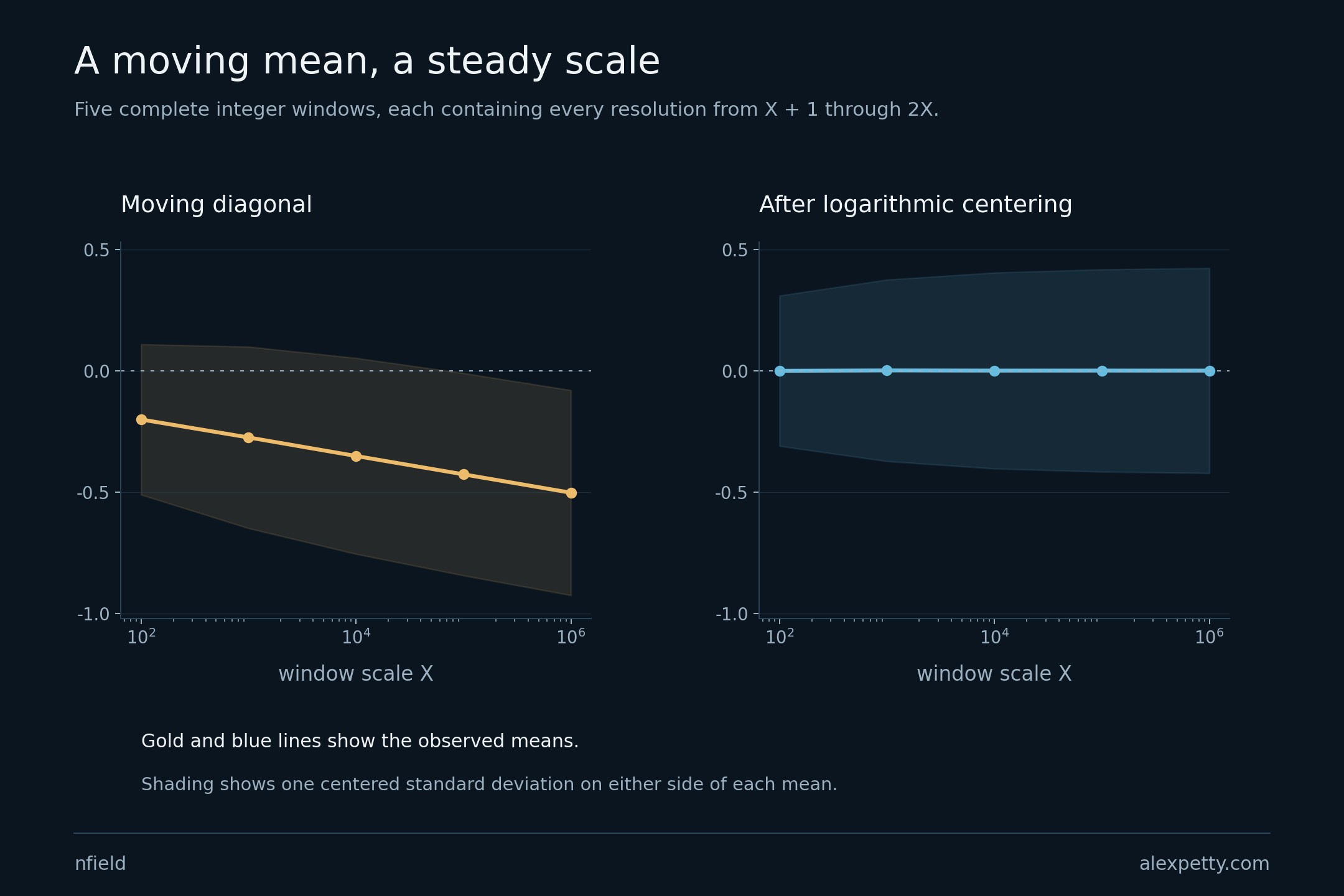
Take all the readings from 1,001 through 2,000. Their average is about $-0.275$. Move to 10,001 through 20,000 and it is $-0.352$. Between one million and two million it is $-0.503$.

The paper accounts for that movement. At integer $n$, the smooth bias is approximately $-0.032853\log n-0.036400$, with the exact constants determined by the weights. Subtract it at each integer. No curve is fitted to the data.

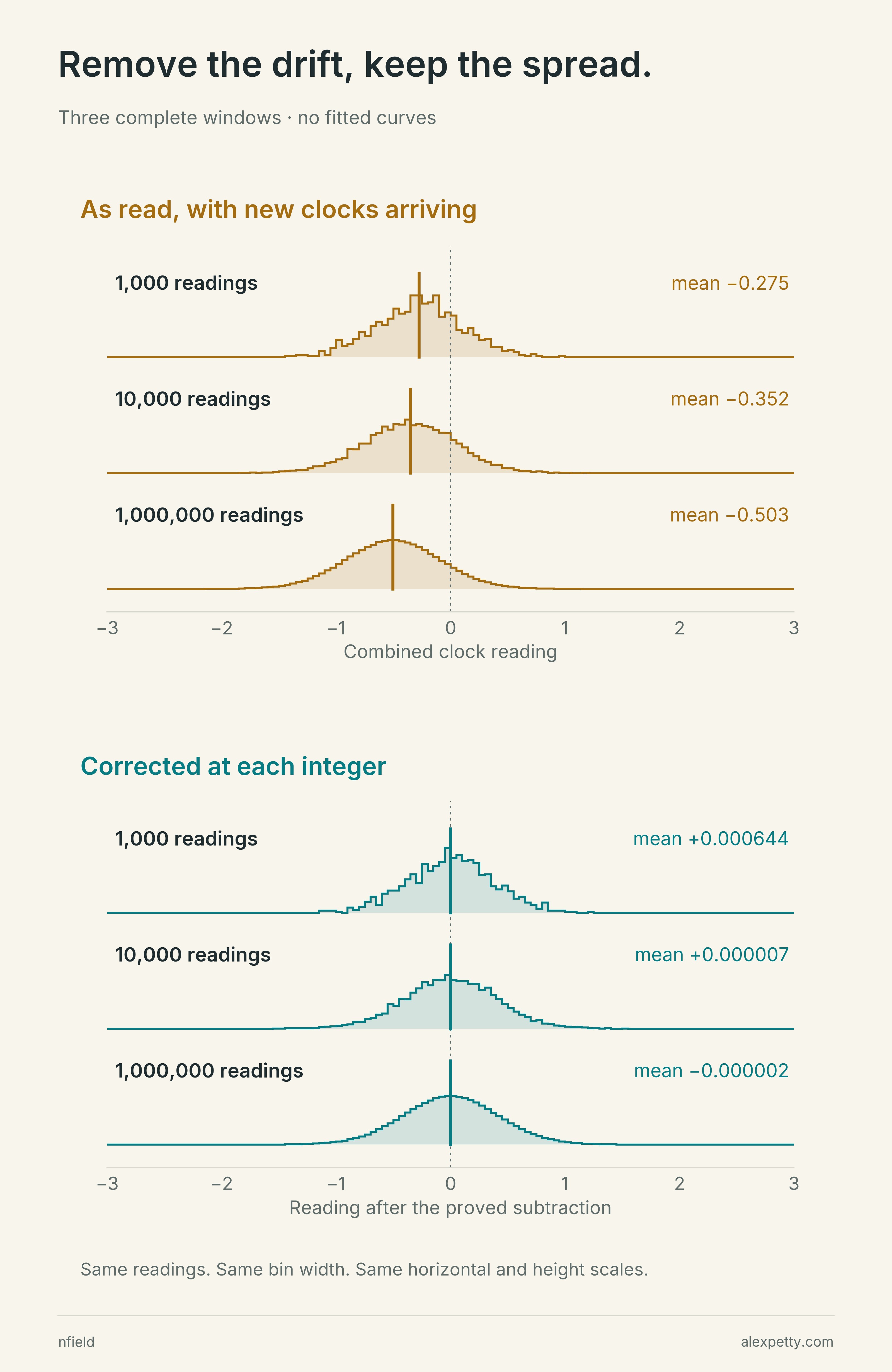
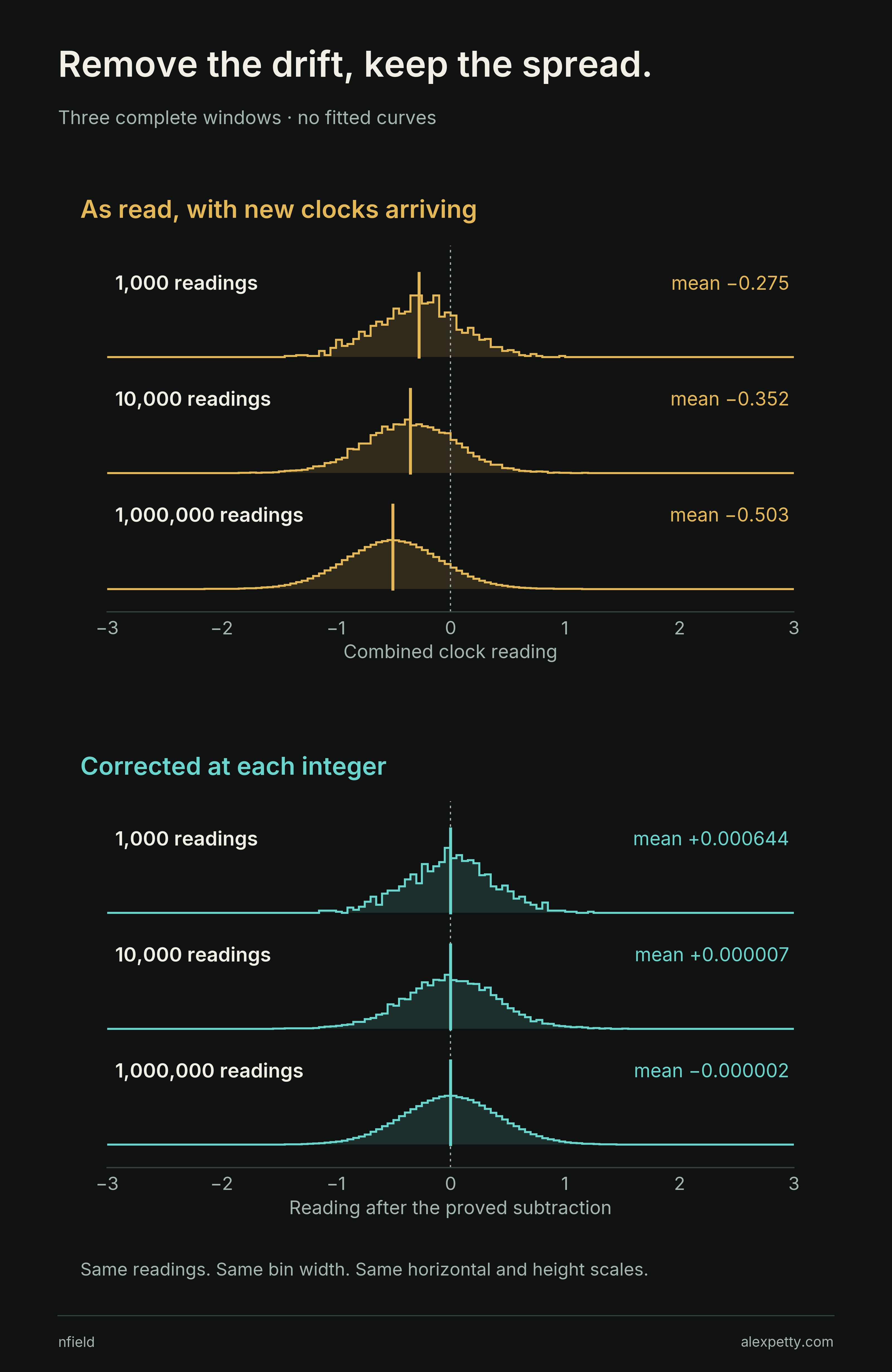
The gold profiles in the figure slide left from window to window, while the teal ones, with the drag removed, stay centered on zero. The corrected readings approach the clock model’s distribution from The Clocks Beneath Collision Energy. Their average square approaches its finite, positive value too. The theorem describes how frequently different readings occur as the observation window moves outward. It does not say that a particular reading settles down.

This is the missing step between the clock model and the calculation. In the model, we average a fixed collection of clocks before enlarging it. Here, every step adds a clock. The proof has to control the whole growing collection at once.

The centering and the transfer theorem

Set $\alpha=1/\zeta(2)$ and

$$\beta=\frac{\gamma}{\zeta(2)} -\frac{\zeta'(2)}{\zeta(2)^2}.$$

The constants come from the cumulative weights and two convergent sawtooth integrals. With

$$\begin{aligned} I_0&=\frac12\log(2\pi)-1,\\ I_1&=1+\frac12\zeta''(0), \end{aligned}$$

they are

$$b=\frac23\alpha I_0,\qquad c=\frac23(\beta I_0-\alpha I_1).$$

Define $Z_n=y_n-b\log n-c$. For an integer chosen uniformly from $X<n\le2X$, the empirical law of $Z_n$ tends to the Haar law of the stationary potential $Y$. The proof also gives

$$\frac1X\sum_{X<n\le2X}Z_n =O\left(X^{-1/3}\log^2(2X)\right)$$

and

$$\begin{gathered} \frac1X\sum_{X<n\le2X}Z_n^2 =\mathbb E Y^2\\ +O\left(X^{-1/5}\log^2(2X)\right). \end{gathered}$$

The main comparison separates short periods, which can be averaged, from long periods, whose combined contribution is evaluated by an integral. A growing range exists where both estimates are small. That overlap is what permits the transfer.

A predictable eight point seven

The same care matters one level up, in the capacity the collision energy is built from. Capacity measures the squared size of the interacting remainder waves. Call it $J(n)$. Its leading profile is $n$, and the shortfall is $D_n=n-J(n)$.

The Secondary Term of the Cubic Law found the main part of that shortfall, $\log^2 n/\pi^2$. At one million that comes to about 19.3. The actual shortfall there is about 28. The clock calculation accounts for the difference.

$$D_n=\frac{\log^2 n}{\pi^2}+B\log n+C+\mathcal R_n.$$

Here $B\approx0.604898$ and $C\approx0.377541$, both given exactly by the weights. At one million, $B\log n+C$ is about 8.7, a smooth and predictable part of the shortfall about twenty times the size of the actual fluctuation, whose typical size near one million is about 0.4. Leave it in, and it buries the thing we are trying to study.

After the full subtraction, the capacity residual $\mathcal R_n$ approaches the same distribution as the corrected clock reading. The two differ by an error that tends to zero.

From the clock reading to capacity

The continuous capacity is exactly

$$J(n)=\frac13\sum_{r,s\le n}\frac{(r,s)^2}{rs},$$

where $(r,s)$ denotes the greatest common divisor. Its deficit includes all periods, including those longer than $n$.

$$D_n=\frac23\sum_{k\ge2}w_k r_k(n).$$

The exact dictionary is

$$D_n=D_*(n)+y_n+\frac{2n}{3}\sum_{k>n}w_k,$$

with $D_*(n)=\frac13\sum_{k\le n}w_k(k-1)$. The omitted long clocks have remainder $n$, which explains the last term. Evaluating the three pieces gives the displayed capacity profile and

$$\mathcal R_n=Z_n+O\left(\frac{\log^2(2n)}n\right).$$

The paper supplies the exact zeta-derivative expressions for $B$ and $C$, rather than estimating them from observed capacities.

The primes sit lower

Prime-base collision energy uses capacity at the preceding integer, $p-1$. Selecting those integers changes which clock positions we see.

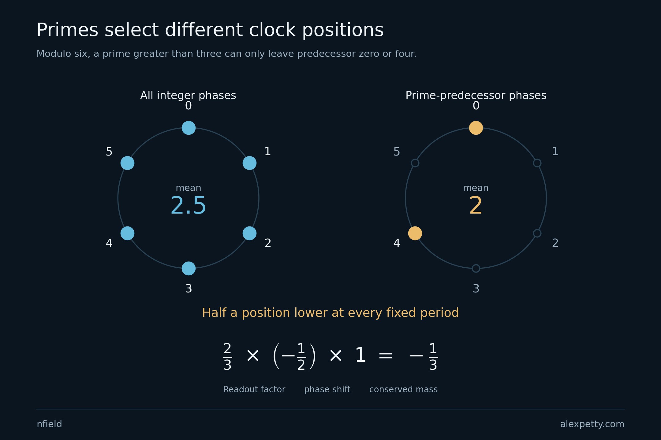
Look at period six. A prime greater than three leaves remainder one or five. Its predecessor therefore leaves zero or four. The average of those two positions is two. The average of all six positions is two and a half.

Half a position lower, before any large computation.

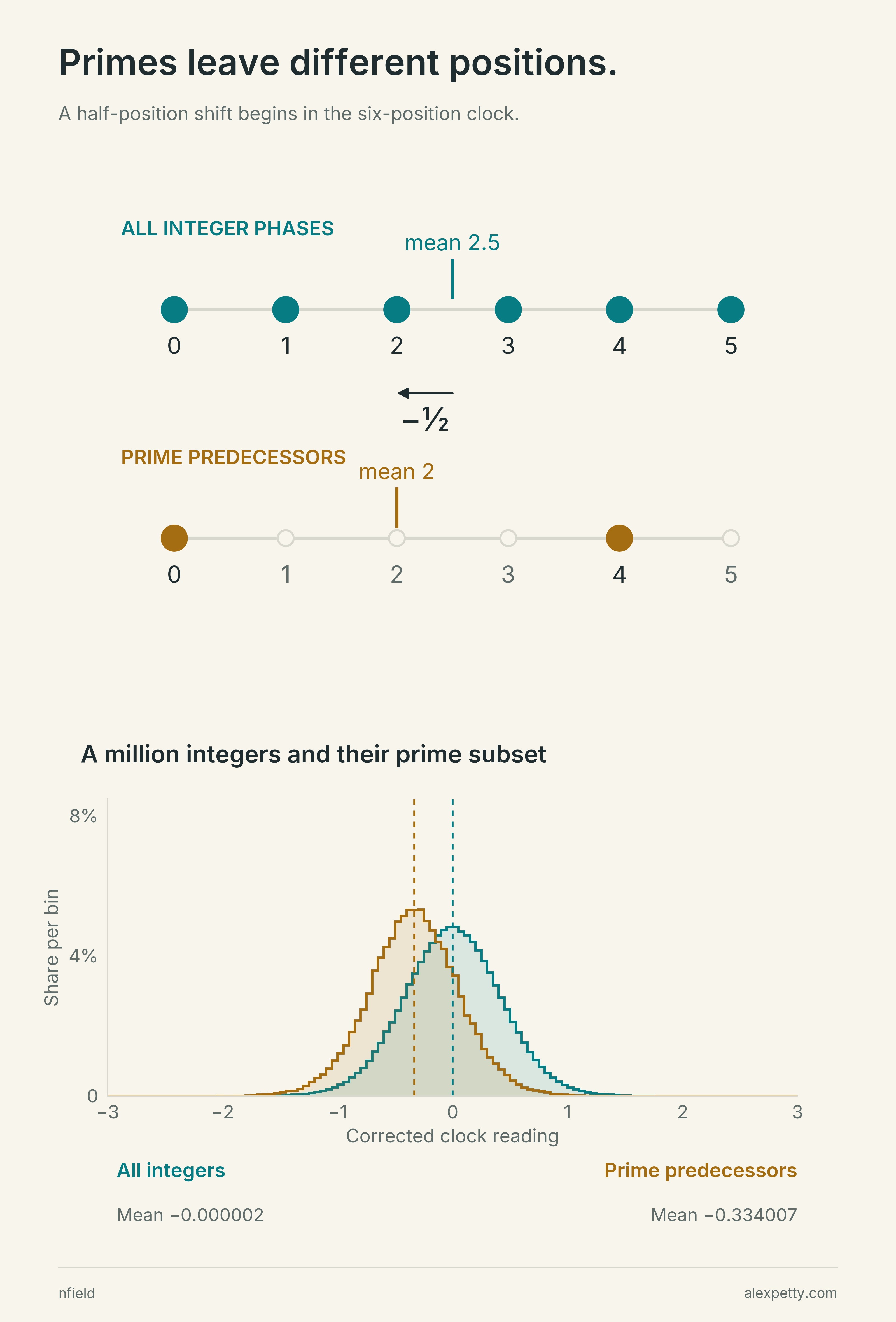
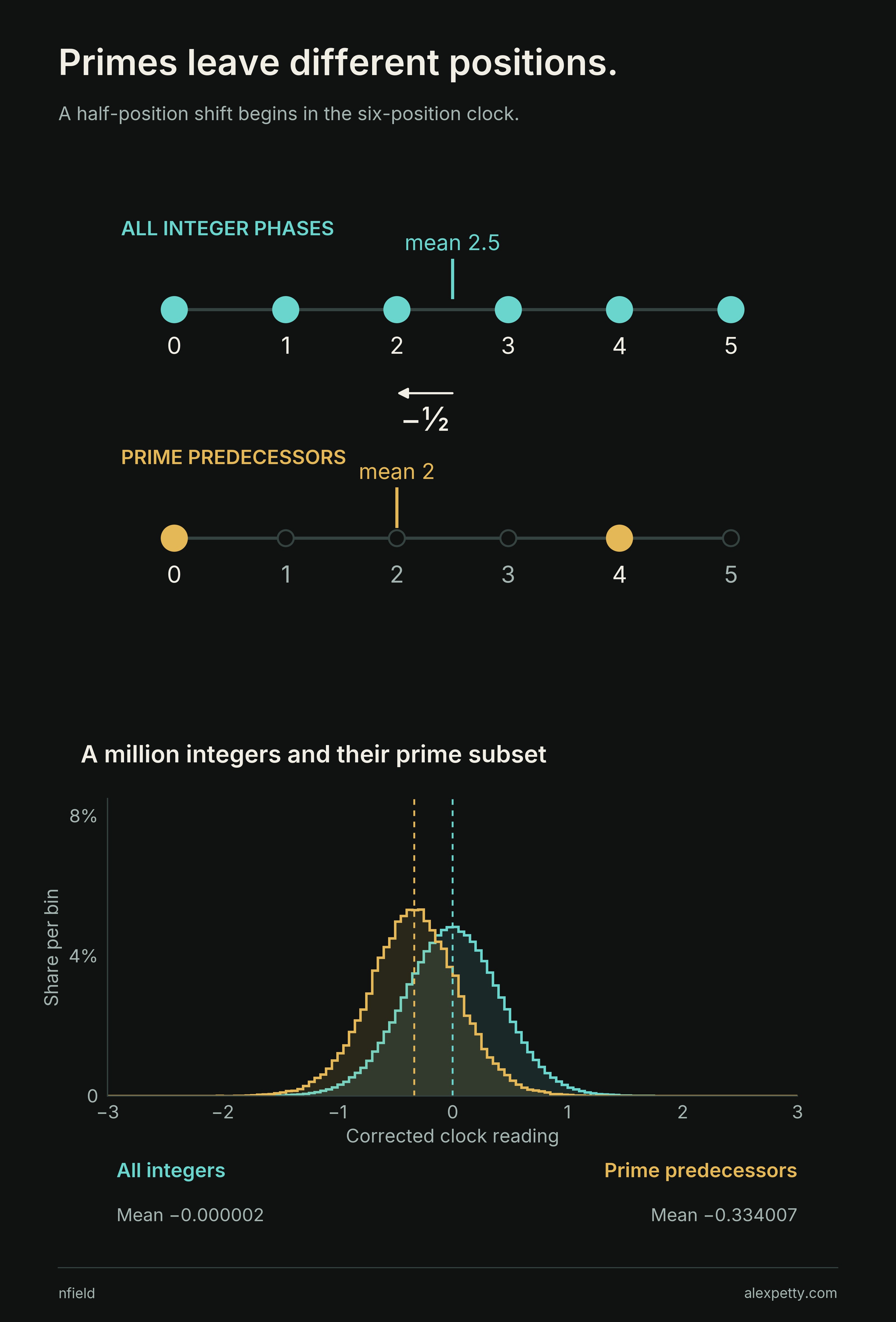
The same half-position shift holds at every fixed period when we average over the allowed prime residue classes. Multiply by the clock readout factor, two thirds, and by the total weight, one. The combined shift is exactly $-1/3$.

A separate argument justifies passing from those residue classes to growing primes. The resulting distribution is symmetric about $-1/3$, with positive finite variance. Moving it right by one third corrects its mean. That does not make it the all-integer distribution.

The result concerns continuous capacity at $p-1$. Transferring this finer law to the original finite digit grid still requires an estimate for the grid-sampling defect.

Half a position lost every period

The units $u$ modulo $k$ pair with $k-u$. Their average least residue is $k/2$, including the single unit at $k=2$. Subtracting one gives predecessor average $k/2-1$, whereas the full clock average is $(k-1)/2$. Their difference is $-1/2$.

For a finite cutoff the mean is therefore

$$-\frac13\sum_{k\le M}w_k.$$

As $M$ grows, this tends to $-1/3$. The paper’s proof constructs the unit-phase limit separately in mean square, then controls growing cutoffs on the prime sample. Its variance is at least $1/324$. The mean, symmetry and nonzero variance are proved, and the plotted window only illustrates them.

The edge draws a parabola

Try a different observation. Keep only the clocks through period $M$ and hold that collection fixed while reading integers from $X+1$ through $2X$. Then choose a larger collection for the next window.

It is tempting to suppose that any cutoff small compared with $X$ will recover the stationary distribution. The unfinished boundary has a more exact requirement. The quantity $M\log M/X$ must tend to zero.

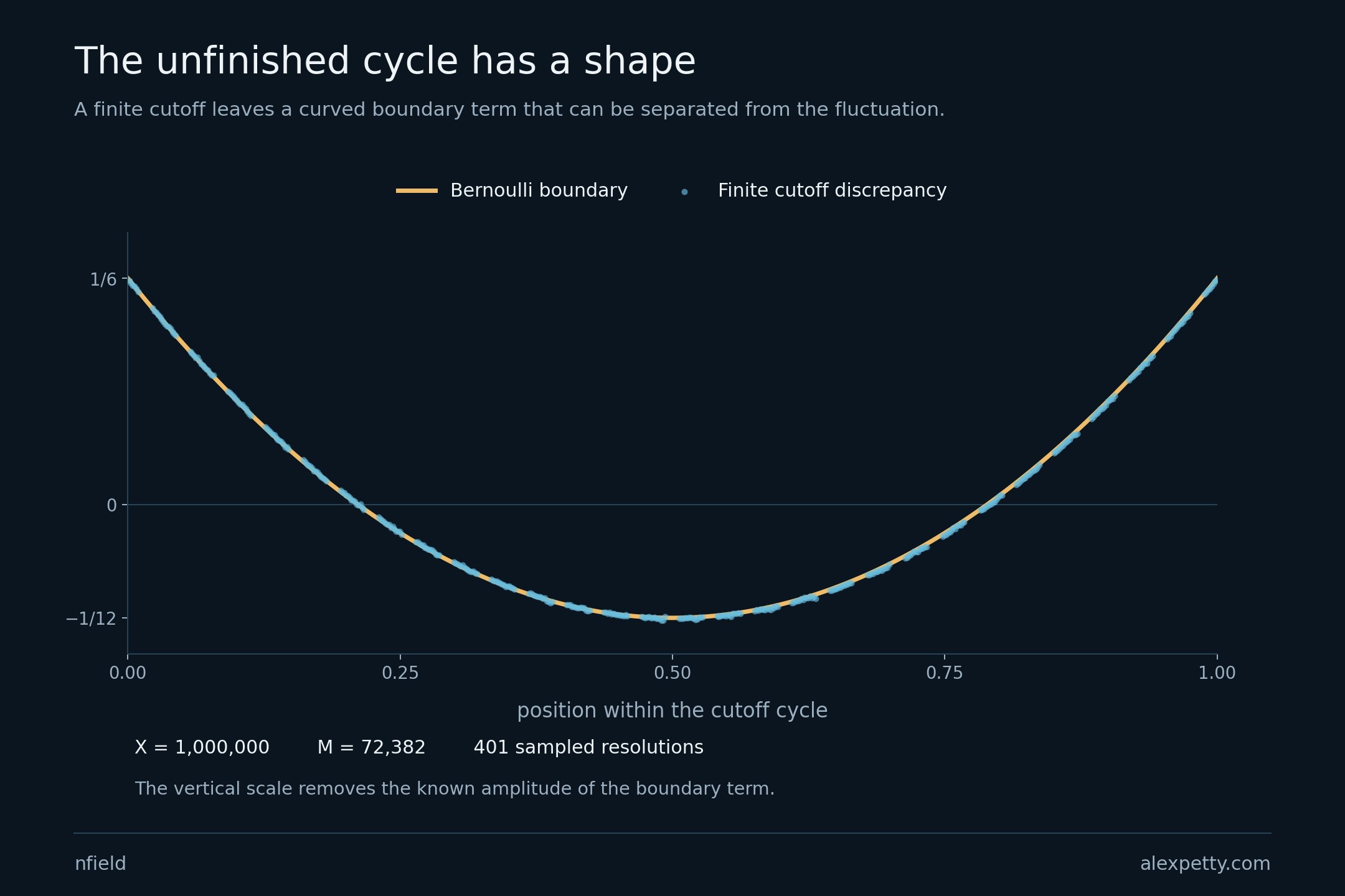
A cutoff near $X/\log X$ is already large enough to contribute a fluctuation of its own. Fold the discrepancy by the cutoff period, bringing each turn onto the same interval. A parabola appears.

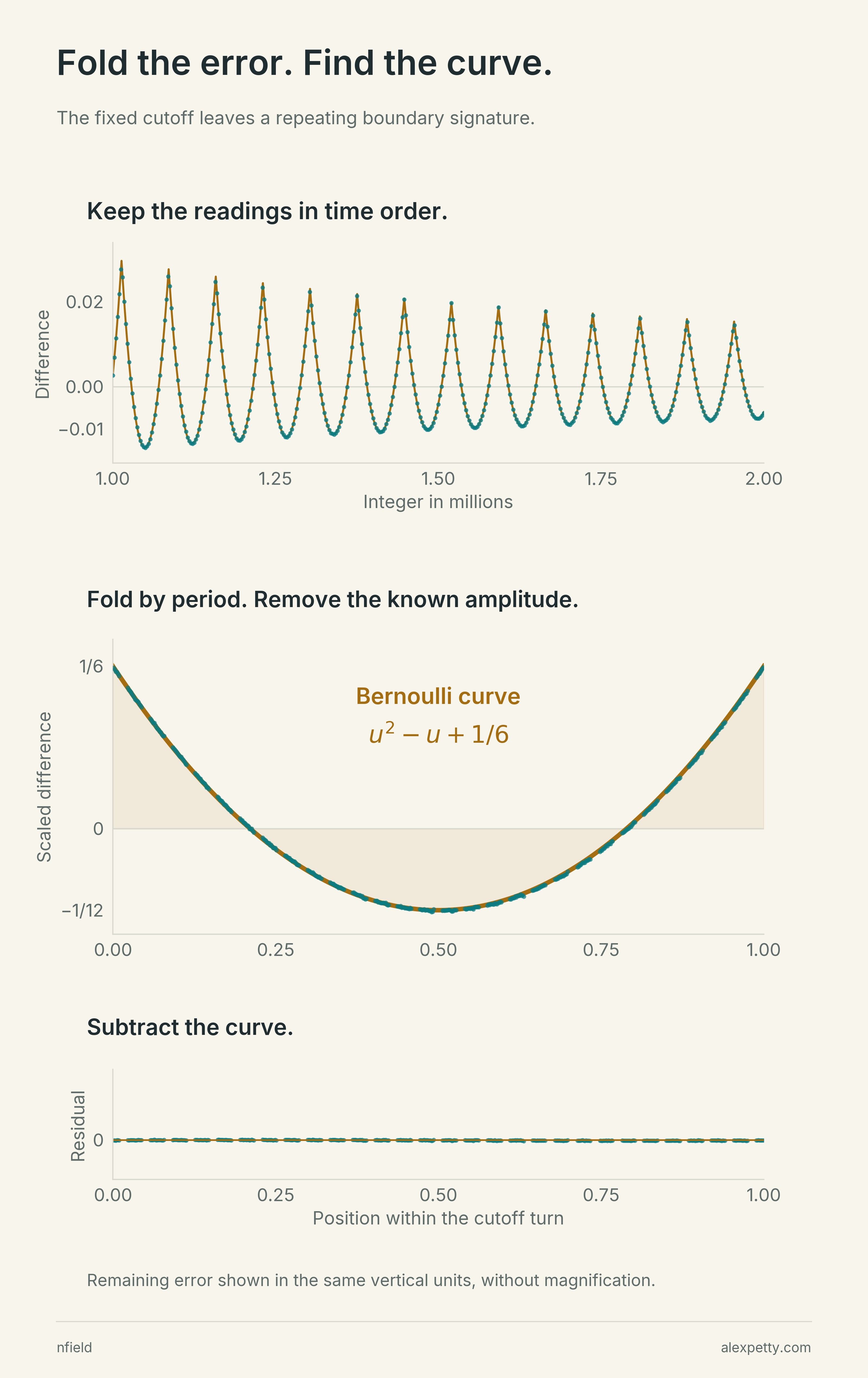
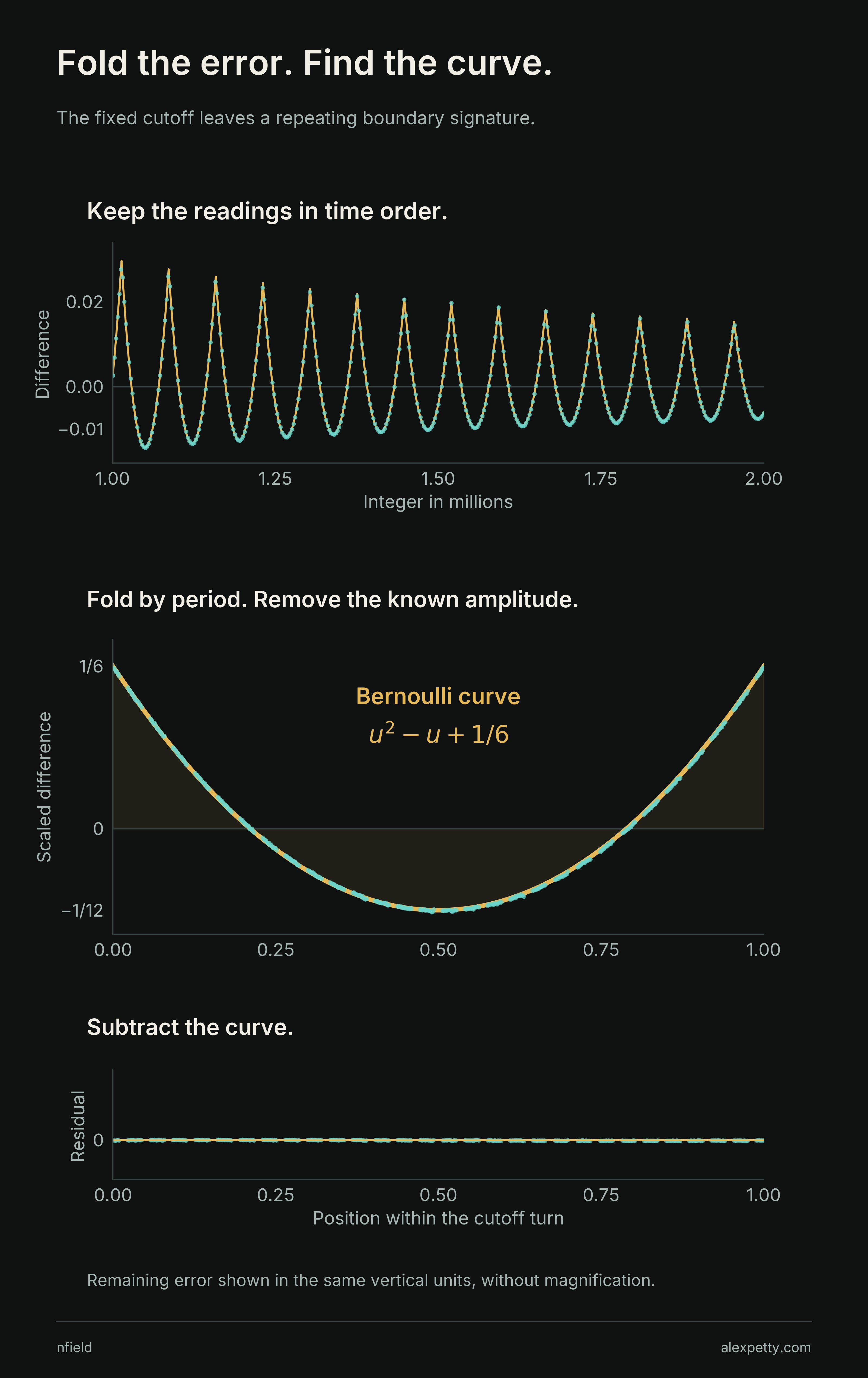
The curve is $u^2-u+1/6$, the second Bernoulli polynomial. The sloping clock reading becomes a quadratic when accumulated. In the proof, integration by parts brings that quadratic to the boundary of the omitted periods.

At the critical scale, this boundary contribution becomes independent of the stationary fluctuation. It adds a precisely calculable amount to the limiting variance. Keeping more clocks has changed the distribution being measured, even though their cutoff remains a vanishing fraction of the observation scale.

The boundary formula and its sharp threshold

Put $u=\{n/M\}$ and $B_2(u)=u^2-u+1/6$. The leading difference is

$$\begin{gathered} Z_n-Y_M(n)\\ =\frac{(\alpha\log M+\beta)M}{3n}B_2(u)\\ +\text{controlled error}. \end{gathered}$$

The figure recomputes the paper’s 401 specified addresses with $X=10^6$ and $M=72\,382$. The root-mean-square discrepancy is about $0.00962$. Subtracting the stated term reduces it to about $0.000117$. No constants are fitted.

Assume $M\to\infty$ and $M=o(X)$. Write $\lambda_X=M\log M/X$. If $\lambda_X\to0$, the stationary law and second moment transfer. If instead $\lambda_X\to\lambda>0$, the frozen-cutoff law tends to

$$Y-\frac{\lambda}{3\zeta(2)T}B_2(U),$$

where $Y$, $T$ and $U$ are independent, $T$ is uniform on $[1,2]$, and $U$ is uniform on $[0,1]$. Its extra second moment is

$$\frac{\lambda^2}{90\pi^4}.$$

If $\lambda_X\to\infty$, the boundary dominates at that scale. Within the stated regime, $M\log M=o(X)$ is necessary and sufficient for the stationary second moment to transfer. The endpoint $M=X$ is a separate regime, not covered by the condition $M=o(X)$.

Watch the admission edge grow

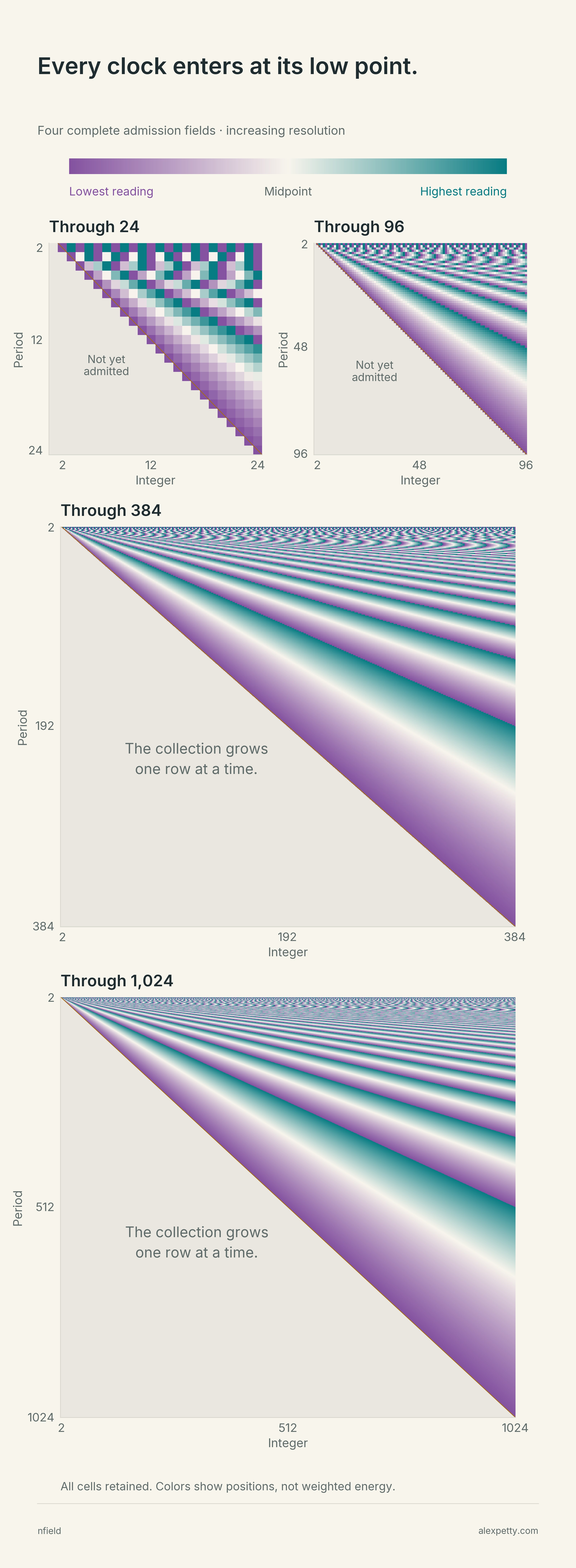
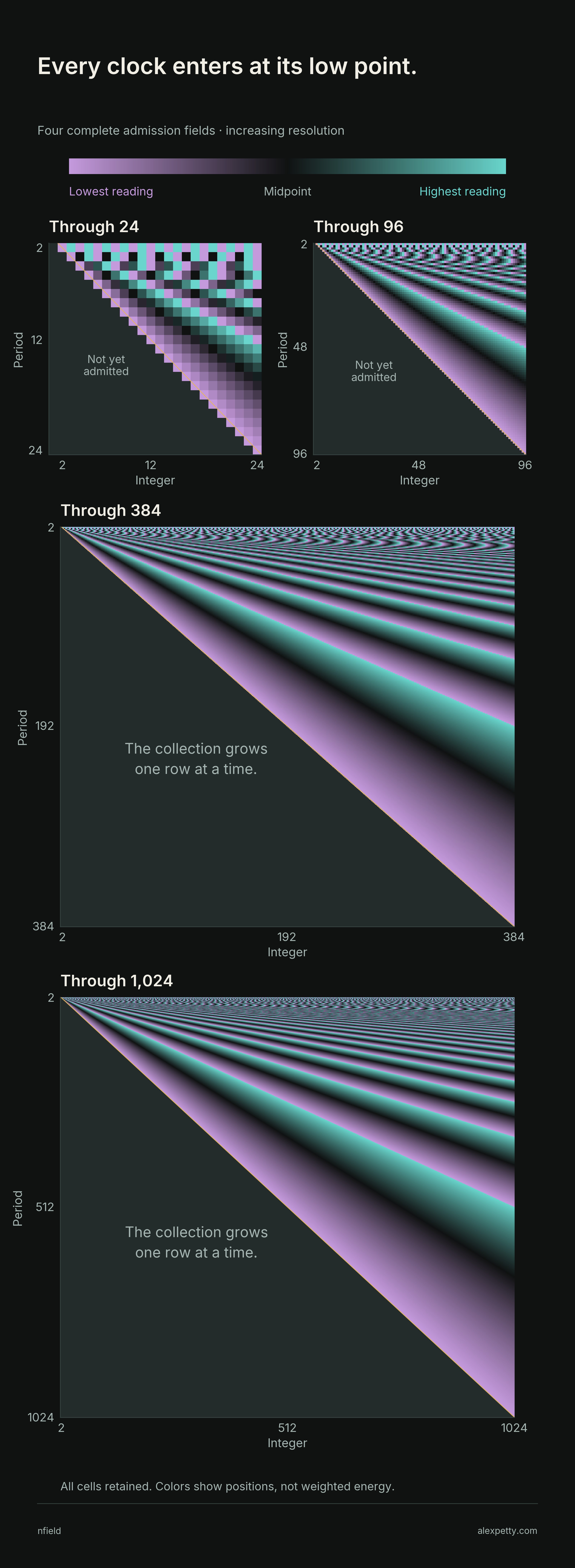
The diagonal separates clocks already admitted from those still waiting. Its first reading is always at the negative end of the color scale. Farther into the field, completed turns leave repeated bands and a fan of reset lines. This is the geometry beneath the cumulative sign identity, with no weights or fitted trend added to the picture.

Four close studies of the clock calculation

The full proofs are in The Stationary-to-Diagonal Transition in Collision Capacity.

A stable distribution still leaves room for rare, large readings. The paper constructs residuals of both signs that grow without bound. They persist even when the contributions from clocks resetting at either neighboring integer are removed.

So the obvious resets do not pay the whole bill. I can describe the limiting spread, and I cannot yet tell you the worst these clocks can do.